Next: 11.5.4 Gaining Information Without Up: 11.5 Examples for Continuous Previous: 11.5.2 Simple Projection Examples
This section illustrates the effect of nature sensing actions, but only for the nondeterministic case. General methods for computing probabilistic I-states are covered in Section 11.6.
 |
 |
Let
![]() . Motions are generated by integrating the velocity
. Motions are generated by integrating the velocity
![]() , which is expressed as
, which is expressed as
![]() and
and
![]() . For simplicity,
assume
. For simplicity,
assume ![]() is applied for all time, which is a command to move
right. The nature action
is applied for all time, which is a command to move
right. The nature action
![]() interferes with the outcome. The robot tries to make progress by
moving in the positive
interferes with the outcome. The robot tries to make progress by
moving in the positive ![]() direction; however, the interference of
nature makes it difficult to predict the
direction; however, the interference of
nature makes it difficult to predict the ![]() direction. Without
nature, there should be no change in the
direction. Without
nature, there should be no change in the ![]() coordinate; however,
with nature, the error in the
coordinate; however,
with nature, the error in the ![]() direction could be as much as
direction could be as much as ![]() ,
after
,
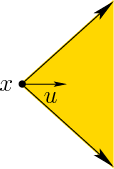
after ![]() seconds have passed. Figure 11.24
illustrates the possible resulting motions.
seconds have passed. Figure 11.24
illustrates the possible resulting motions.
Sensor observations will be made that alleviate the growing cone of
uncertainty; use the sensing model from Figure 11.11, and
suppose that the measurement error ![]() is
is ![]() . Suppose there is a
disc in
. Suppose there is a
disc in
![]() of radius larger than
of radius larger than ![]() , as shown in Figure
11.23a. Since the true state is never further than
, as shown in Figure
11.23a. Since the true state is never further than
![]() from the measured state, it is always possible to determine
whether the state passed above or below the disc. Multiple possible
observation histories are shown in Figure 11.23a.
The observation history need not even be continuous, but it is drawn
that way for convenience. For a disc with radius less than
from the measured state, it is always possible to determine
whether the state passed above or below the disc. Multiple possible
observation histories are shown in Figure 11.23a.
The observation history need not even be continuous, but it is drawn
that way for convenience. For a disc with radius less than ![]() , there
may exist some observation histories for which it is impossible to
determine whether the true state traveled above or below the disc; see
Figure 11.23b. For other observation histories, it
may still be possible to make the determination; for example, from the
uppermost trajectory shown in Figure 11.23b it is
known for certain that the true state traveled above the disc.
, there
may exist some observation histories for which it is impossible to
determine whether the true state traveled above or below the disc; see
Figure 11.23b. For other observation histories, it
may still be possible to make the determination; for example, from the
uppermost trajectory shown in Figure 11.23b it is
known for certain that the true state traveled above the disc.
![]()
 |
To control the robot, a motion command is given in the form of an
action
![]() . Nature interferes with the motions in two
ways: 1) The robot tries to travel some distance
. Nature interferes with the motions in two
ways: 1) The robot tries to travel some distance ![]() , but there is
some error
, but there is
some error
![]() , for which the true distance traveled,
, for which the true distance traveled,
![]() , is known satisfy
, is known satisfy
![]() ; and 2) the
robot tries to move in a direction
; and 2) the
robot tries to move in a direction ![]() , but there is some error,
, but there is some error,
![]() , for which the true direction
, for which the true direction ![]() is known to
satisfy
is known to
satisfy
![]() . These two independent errors
can be modeled by defining a 2D nature action set,
. These two independent errors
can be modeled by defining a 2D nature action set, ![]() . The
transition equation is then defined so that the forward projection
. The
transition equation is then defined so that the forward projection
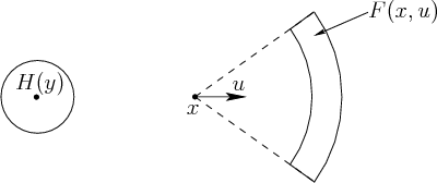
![]() is as shown in Figure 11.25.
is as shown in Figure 11.25.
 |
Some nondeterministic I-states will now be constructed. Suppose that
the initial state ![]() is known, and history I-states take the form
is known, and history I-states take the form
| (11.73) |
The next step is considerably more complicated. Suppose that ![]() and that (11.30) is applied to compute
and that (11.30) is applied to compute
![]() from
from
![]() . The shape shown in Figure
11.26c is obtained by taking the union of
. The shape shown in Figure
11.26c is obtained by taking the union of
![]() for
all possible
for
all possible
![]() . The resulting shape is composed
of circular arcs and straight line segments (see Exercise
13). Once
. The resulting shape is composed
of circular arcs and straight line segments (see Exercise
13). Once ![]() is obtained, an intersection is taken
once again to yield
is obtained, an intersection is taken
once again to yield
![]() , as
shown in Figure 11.27. The process repeats in the same way
for the desired number of stages. The complexity of the region in
Figure 11.26c provides motivation for the approximation
methods of Section 11.4.3. For example, the
nondeterministic I-states could be nicely approximated by ellipsoidal
regions.
, as
shown in Figure 11.27. The process repeats in the same way
for the desired number of stages. The complexity of the region in
Figure 11.26c provides motivation for the approximation
methods of Section 11.4.3. For example, the
nondeterministic I-states could be nicely approximated by ellipsoidal
regions.
![]()
Steven M LaValle 2020-08-14