Linear sensing models

Developed mainly in control theory literature, linear sensing models are some of the most common and important. For all of the sensors in this family, assume that $X = Y = {\mathbb{R}}^n$ (nonsingular linear transformations allow the sensor space to effectively have lower dimension, if desired). The simplest case in this family is the identity sensor, in which $y = x$. In this case, the state is immediately known. If this sensor is available at every stage, then the I-space collapses to $X$ by the I-map ${{\kappa}_{sf}}: {\cal I}_{hist} \rightarrow X$.

Figure 11.11: A simple sensing model in which the observation error is no more than $r$: (a) the nature sensing action space; (b) the preimage in $X$ based on observation $y$.

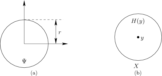
Now nature sensing actions can be used to corrupt this perfect state observation to obtain $y = h(x,\psi) = x + \psi$. Suppose that $y$ is an estimate of $x$, the current state, with error bounded by a constant $r \in (0,\infty)$. This can be modeled by assigning for every $x \in X$, $\Psi(x)$ as a closed ball of radius $r$, centered at the origin:

$$\Psi = \{\psi \in {\mathbb{R}}^n \;\vert\; \Vert\psi\Vert \leq r\} .$$ (11.67)

Figure 11.11 illustrates the resulting nondeterministic sensing model. If the observation $y$ is received, then it is known that the true state lies within a ball in $X$ of radius $r$, centered at $y$. This ball is the preimage, $H(y)$, as defined in (11.11). To make the model probabilistic, a probability density function can be defined over $\Psi$. For example, it could be assumed that $p(\psi)$ is a uniform density (although this model is not very realistic in many applications because there is a boundary at which the probability mass discontinuously jumps to zero).

A more typical probabilistic sensing model can be made by letting $\Psi(x) = {\mathbb{R}}^n$ and defining a probability density function over all of ${\mathbb{R}}^n$. (Note that the nondeterministic version of this sensor is completely useless.) One of the easiest choices to work with is the multivariate Gaussian probability density function,

$$p(\psi) = \frac{1}{\sqrt{(2\pi)^n\vert\Sigma\vert}} e^{-\frac{1}{2} \psi^T \Sigma \psi} ,$$ (11.68)

in which $\Sigma$ is the covariance matrix (11.64), $\vert\Sigma\vert$ is its determinant, and $\psi^T \Sigma \psi$ is a quadratic form, which multiplies out to yield

$$\psi^T \Sigma \psi = \sum_{i=1}^n \sum_{j=1}^n \sigma_{i,j} \psi_i \psi_j .$$ (11.69)

If $p(x)$ is a Gaussian and $y$ is received, then $p(y\vert x)$ must also be Gaussian under this model. This will become very important in Section 11.6.1.

The sensing models presented so far can be generalized by applying linear transformations. For example, let $C$ denote a nonsingular $n \times n$ matrix with real-valued entries. If the sensor mapping is $y = h(x) = C x$, then the state can still be determined immediately because the mapping $y = C x$ is bijective; each $H(y)$ contains a unique point of $X$. A linear transformation can also be formed on the nature sensing action. Let $W$ denote an $n \times n$ matrix. The sensor mapping is

$$y = h(x) = C x + W \psi .$$ (11.70)

In general, $C$ and $W$ may even be singular, and a linear sensing model is still obtained. Suppose that $W = 0$. If $C$ is singular, however, it is impossible to infer the state directly from a single sensor observation. This generally corresponds to a projection from an $n$-dimensional state space to a subset of $Y$ whose dimension is the rank of $C$. For example, if

$$C = \begin{pmatrix}0 & 1 0 & 0 \end{pmatrix} ,$$ (11.71)

then $y = C x$ yields $y_1 = x_2$ and $y_2 = 0$. Only $x_2$ of each $(x_1,x_2) \in X$ can be observed because $C$ has rank $1$. Thus, for some special cases, singular matrices can measure some state variables while leaving others invisible. For a general singular matrix $C$, the interpretation is that $X$ is projected into some $k$-dimensional subspace by the sensor, in which $k$ is the rank of $C$. If $W$ is singular, this means that the effect of nature is limited. The degrees of freedom with which nature can distort the sensor observations is the rank of $W$. These concepts motivate the next set of sensor models.