14.5.2 Dynamic Programming with Interpolation

As observed in Section 14.4, motion planning under differential constraints is extremely challenging. Additionally requiring feedback complicates the problem even further. If ${X_{obs}}= \emptyset$, then a feedback plan can be designed using numerous techniques from control theory. See Section 15.2.2 and [192,523,846]. In many cases, designing feedback plans is no more difficult than computing an open-loop trajectory. However, if ${X_{obs}}\not = \emptyset$, feedback usually makes the problem much harder.

Fortunately, dynamic programming once again comes to the rescue. In Section 2.3, value iteration yielded feedback plans for discrete state spaces and state transition equations. It is remarkable that this idea can be generalized to the case in which $U$ and $X$ are continuous and there is a continuum of stages (called time). Most of the tools required to apply dynamic programming in the current setting were already introduced in Section 8.5.2. The main ideas in that section were to represent the optimal cost-to-go $G^*$ by interpolation and to use a discrete-time approximation to the motion planning problem.

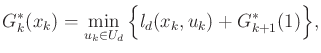
The discrete-time model of Section 14.2.2 can be used in the current setting to obtain a discrete-stage state transition equation of the form $x_{k+1} = f_d(x_k,u_k)$. The cost functional is approximated as in Section 8.5.2 by using (8.65). This integral can be evaluated numerically by using the result of the system simulator and yields the cost-per-stage as $l_d(x_k,u_k)$. Using backward value iteration, the dynamic programming recurrence is

$$G^*_k({x_k}) = \min_{{u_k}\in U_d} \Big\{ l_d({x_k},{u_k}) + G^*_{k+1}(\xkp1) \Big\} ,$$ (14.27)

which is similar to (2.11) and (8.56). The finite set $U_d$ of action samples is used if $U$ is not already finite. The system simulator is applied to determine whether some points along the trajectory lie in ${X_{obs}}$. In this case, $l_d(x_k,u_k) = \infty$, which prevents actions from being chosen that violate constraints.

As in Section 8.5.2, a set $P \subset X$ of samples is used to approximate $G^*$ over $X$. The required values at points in $X \setminus P$ are obtained by interpolation. For example, the barycentric subdivision scheme of Figure 8.20 may be applied here to interpolate over simplexes in $O(n \lg n)$ time, in which $n$ is the dimension of $X$.

As usual, backward value iteration starts at some final stage $F$ and proceeds backward through the stage indices. Termination occurs when all of the cost-to-go values stabilize. The initialization at stage $F$ yields $G^*_F(x) = 0$ for $x \in {X_{G}}\cap P$; otherwise, $G^*_F(x) = \infty$. Each subsequent iteration is performed by evaluating (14.27) on each $x \in P$ and using interpolation to obtain $G^*_{k+1}(\xkp1)$.

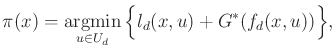
The resulting stationary cost-to-go function $G^*$ can serve as a navigation function over ${X_{free}}$, as described in Section 8.5.2. Recall from Chapter 8 that a navigation function is converted into a feedback plan by applying a local operator. The local operator in the present setting is

$$\pi (x) = \operatornamewithlimits{argmin}_{u \in U_d} \Big\{ l_d(x,u) + G^*(f_d(x,u)) \Big\} ,$$ (14.28)

which yields an action for any state in ${X_{free}}$ that falls into an interpolation neighborhood of some samples in $P$.

Unfortunately, the method presented here is only useful in spaces of a few dimensions. If $X = {\cal C}$, then it may be applied, for example, to the systems in Section 13.1.2. If dynamics are considered, then in many circumstances the dimension is too high because the dimension of $X$ is usually twice that of ${\cal C}$. For example, if ${\cal A}$ is a rigid body in the plane, then the dimension of $X$ is six, which is already at the usual limit of practical use.

It is interesting to compare the use of dynamic programming here with that of Sections 14.4.1 and 14.4.2, in which a search graph was constructed. If Dijkstra's algorithm is used (or even breadth-first search in the case of time optimality), then by the dynamic programming principle, the resulting solutions are approximately optimal. To ensure convergence, resolution completeness arguments were given based on Lipschitz conditions on $f$. It was important to allow the resolution to improve as the search failed to find a solution. Instead of computing a search graph, value iteration is based on computing cost-to-go functions. In the same way that both forward and backward versions of the tree-based approaches were possible, both forward and backward value iteration can be used here. Providing resolution completeness is more difficult, however, because ${x_{I}}$ is not fixed. It is therefore not known whether some resolution is good enough for the intended application. If ${x_{I}}$ is known, then $G^*$ can be used to generate a trajectory from ${x_{I}}$ using the system simulator. If the trajectory fails to reach ${X_{G}}$, then the resolution can be improved by adding more samples to $P$ and $U_d$ or by reducing $\Delta t$. Under Lipschitz conditions on $f$, the approach converges to the true optimal cost-to-go [92,168,565]. Therefore, value iteration can be considered resolution complete with respect to a given ${x_{I}}$. The convergence even extends to computing optimal feedback plans with additional actions that are taken by nature, which is modeled nondeterministically or probabilistically. This extends the value iteration method of Section 10.6.

The relationship between the methods based on a search graph and on value iteration can be brought even closer by constructing Dijkstra-like versions of value iteration, as described at the end of Section 8.5.2. These extend Dijkstra's algorithm, which was viewed for the finite case in Section 2.3.3 as an improvement to value iteration. The improvement to value iteration is made by recognizing that in most evaluations of (14.27), the cost-to-go value does not change. This is caused by two factors: 1) From some states, no trajectory has yet been found that leads to ${X_{G}}$; therefore, the cost-to-go remains at infinity. 2) The optimal cost-to-go from some state might already be computed; no future iterations would improve the cost.

A forward or backward version of a Dijkstra-like algorithm can be made. Consider the backward case. The notion of a backprojection was used in Section 8.5.2 to characterize the set of states that can reach another set of states in one stage. This was used in (8.68) to define the frontier during the execution of the Dijkstra-like algorithm. There is essentially no difference in the current setting to handle the system ${\dot x}= f(x,u)$. Once the discrete-time approximation has been made, the definition of the backprojection is essentially the same as in (8.66) of Section 8.5.2. Using the discrete-time model of Section 14.2.2, the backprojection of a state $x \in {X_{free}}$ is

$$\operatorname{B}(x) = \{x' \in {X_{free}}\;\vert\; \exists u \in U_d x = f_d(x',u)\}.$$ (14.29)

The backprojection is closely related to the backward time-limited reachable set from Section 14.2.1. The backprojection can be considered as a discrete, one-stage version, which indicates the states that can reach $x$ through the application of a constant action $u \in U_d$ over time $\Delta t$. As mentioned in Section 8.5.2, computing an overapproximation to the frontier set may be preferable in practice. This can be obtained by approximating the backprojections, which are generally more complicated under differential constraints than for the case considered in Section 8.5.2. One useful simplification is to ignore collisions with obstacles in defining $\operatorname{B}(x)$. Also, a simple bounding volume of the true backprojection may be used. The trade-offs are similar to those in collision detection, as mentioned in Section 5.3.2. Sometimes the structure of the particular system greatly helps in determining the backprojections. A nice wavefront propagation algorithm can be obtained, for example, for a double integrator; this is exploited in Section 14.6.3. For more on value iteration and Dijkstra-like versions, see [607].