2.3.1.1 Backward value iteration

As for the search methods, there are both forward and backward versions of the approach. The backward case will be covered first. Even though it may appear superficially to be easier to progress from ${x_{I}}$, it turns out that progressing backward from ${X_{G}}$ is notationally simpler. The forward case will then be covered once some additional notation is introduced.

The key to deriving long optimal plans from shorter ones lies in the construction of optimal cost-to-go functions over $X$. For $k$ from $1$ to $F$, let $G^*_k$ denote the cost that accumulates from stage $k$ to $F$ under the execution of the optimal plan:

$$G^*_k(x_k) = \min_{u_k,\ldots,u_K} \left\{ \sum_{i=k}^{K} l(x_i,u_i) + l_F(x_F) \right\} .$$ (2.5)

Inside of the $\min$ of (2.5) are the last $F-k$ terms of the cost functional, (2.4). The optimal cost-to-go for the boundary condition of $k = F$ reduces to

$$G^*_F(x_F) = l_F(x_F) .$$ (2.6)

This makes intuitive sense: Since there are no stages in which an action can be applied, the final stage cost is immediately received.

Now consider an algorithm that makes $K$ passes over $X$, each time computing $G^*_k$ from $G^*_{k+1}$, as $k$ ranges from $F$ down to $1$. In the first iteration, $G^*_F$ is copied from $l_F$ without significant effort. In the second iteration, $G^*_K$ is computed for each $x_K \in X$ as

$$G^*_K(x_K) = \min_{u_K} \Big\{ l(x_K,u_K) + l_F(x_F) \Big\} .$$ (2.7)

Since $l_F = G^*_F$ and $x_F = f(x_K,u_K)$, substitutions can be made into (2.7) to obtain

$$G^*_K(x_K) = \min_{u_K} \Big\{ l(x_K,u_K) + G^*_F(f(x_K,u_K)) \Big\},$$ (2.8)

which is straightforward to compute for each $x_K \in X$. This computes the costs of all optimal one-step plans from stage $K$ to stage $F = K+1$.

It will be shown next that $G^*_k$ can be computed similarly once $G^*_{k+1}$ is given. Carefully study (2.5) and note that it can be written as

$$G^*_k(x_k) = \min_{{u_k}} \left\{ \min_{\ukp1, \ldots, {u_K}} \left\{ l({x_k},{u_k}) + \sum_{i=k+1}^K l({x_i},{u_i}) + l_F(\xKp1) \right\} \right\}$$ (2.9)

by pulling the first term out of the sum and by separating the minimization over ${u_k}$ from the rest, which range from $u_{k+1}$ to $u_K$. The second $\min$ does not affect the $l({x_k},{u_k})$ term; thus, $l({x_k},{u_k})$ can be pulled outside to obtain

$$G^*_k({x_k}) = \min_{{u_k}} \left\{ l({x_k},{u_k}) + \min_{\ukp1,... ..., {u_K}} \left\{ \sum_{i=k+1}^K l({x_i},{u_i}) + l_F(\xKp1) \right\} \right\} .$$ (2.10)

The inner $\min$ is exactly the definition of the optimal cost-to-go function $G^*_{k+1}$. Upon substitution, this yields the recurrence

$$G^*_k({x_k}) = \min_{{u_k}} \Big\{ l({x_k},{u_k}) + G^*_{k+1}(\xkp1) \Big\} ,$$ (2.11)

in which $x_{k+1} = f({x_k},{u_k})$. Now that the right side of (2.11) depends only on ${x_k}$, ${u_k}$, and $G^*_{k+1}$, the computation of $G^*_k$ easily proceeds in $O(\vert X\vert \vert U\vert)$ time. This computation is called a value iteration. Note that in each value iteration, some states receive an infinite value only because they are not reachable; a $(K-k)$-step plan from $x_k$ to ${X_{G}}$ does not exist. This means that there are no actions, $u_k \in U(x_k)$, that bring $x_k$ to a state $x_{k+1} \in X$ from which a $(K-k-1)$-step plan exists that terminates in ${X_{G}}$.

Summarizing, the value iterations proceed as follows:

$$G^*_F \;\;\rightarrow \;\; G^*_K \;\;\rightarrow\;\; G^*_{K-1} \;... ... \;\;\rightarrow\;\; G^*_{k-1} \;\; \cdots \;\; G^*_2 \;\;\rightarrow\;\; G^*_1$$ (2.12)

until finally $G^*_1$ is determined after $O(K \vert X\vert \vert U\vert)$ time. The resulting $G^*_1$ may be applied to yield $G^*_1({x_{I}})$, the optimal cost to go to the goal from ${x_{I}}$. It also conveniently gives the optimal cost-to-go from any other initial state. This cost is infinity for states from which ${X_{G}}$ cannot be reached in $K$ stages.

It seems convenient that the cost of the optimal plan can be computed so easily, but how is the actual plan extracted? One possibility is to store the action that satisfied the $\min$ in (2.11) from every state, and at every stage. Unfortunately, this requires $O(K \vert X\vert)$ storage, but it can be reduced to $O(\vert X\vert)$ using the tricks to come in Section 2.3.2 for the more general case of variable-length plans.

Example 2..3 (A Five-State Optimal Planning Problem)   Figure 2.8 shows a graph representation of a planning problem in which $X = \{a,c,b,d,e\}$. Suppose that $K=4$, ${x_{I}}= a$, and ${X_{G}}= \{d\}$. There will hence be four value iterations, which construct $G^*_4$, $G^*_3$, $G^*_2$, and $G^*_1$, once the final-stage cost-to-go, $G^*_5$, is given.

Figure 2.8: A five-state example. Each vertex represents a state, and each edge represents an input that can be applied to the state transition equation to change the state. The weights on the edges represent $l(x_k,u_k)$ ($x_k$ is the originating vertex of the edge).

Figure 2.9: The optimal cost-to-go functions computed by backward value iteration.

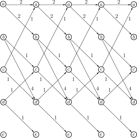
Figure 2.10: The possibilities for advancing forward one stage. This is obtained by making two copies of the states from Figure 2.8, one copy for the current state and one for the potential next state.

Figure 2.11: By turning Figure 2.10 sideways and copying it $K$ times, a graph can be drawn that easily shows all of the ways to arrive at a final state from an initial state by flowing from left to right. The computations automatically select the optimal route.

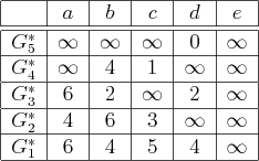
The cost-to-go functions are shown in Figure 2.9. Figures 2.10 and 2.11 illustrate the computations. For computing $G^*_4$, only $b$ and $c$ receive finite values because only they can reach $d$ in one stage. For computing $G^*_3$, only the values $G^*_4(b) = 4$ and $G^*_4(c) = 1$ are important. Only paths that reach $b$ or $c$ can possibly lead to $d$ in stage $k=5$. Note that the minimization in $(\ref{eqn:ctgk2})$ always chooses the action that produces the lowest total cost when arriving at a vertex in the next stage. $\blacksquare$