14.4.3 RDT-Based Methods

The rapidly exploring dense tree (RDT) family of methods, which includes the RRT, avoids maintaining a lattice altogether. RDTs were originally developed for handling differential constraints, even though most of their practical application has been to the Piano Mover's Problem. This section extends the ideas of Section 5.5 from ${\cal C}$ to $X$ and incorporates differential constraints. The methods covered so far in Section 14.4 produce approximately optimal solutions if the graph is searched using dynamic programming and the resolution is high enough. By contrast, RDTs are aimed at returning only feasible trajectories, even as the resolution improves. They are often successful at producing a solution trajectory with relatively less sampling. This performance gain is enabled in part by the lack of concern for optimality.

Let ${\alpha }$ denote an infinite, dense sequence of samples in $X$. Let $\rho: X \times X \rightarrow [0,\infty]$ denote a distance function on $X$, which may or may not be a proper metric. The distance function may not be symmetric, in which case $\rho(x_1,x_2)$ represents the directed distance from $x_1$ to $x_2$.

The RDT is a search graph as considered so far in this section and can hence be interpreted as a subgraph of the reachability graph under some discretization model. For simplicity, first assume that the discrete-time model of Section 14.2.2 is used, which leads to a finite action set $U_d$ and a fixed time interval $\Delta t$. The set ${\cal U}^p$ of motion primitives is all action trajectories for which some $u \in U_d$ is held constant from time 0 to $\Delta t$. The more general case will be handled at the end of this section.

Figure 14.19: Extending the basic RDT algorithm to handle differential constraints. In comparison to Figure 5.16, an LPM computes $x_r$, which becomes the new vertex, instead of ${\alpha }(i)$. In some applications, line 4 may fail, in which case lines 5 and 6 are skipped.

Figure 14.20: If the nearest point $S$ lies in the state trajectory segment associated to an edge, then the edge is split into two, and a new vertex is inserted into ${\cal G}$.

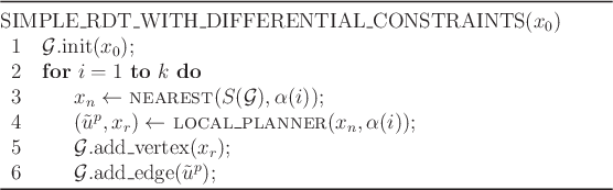
Paralleling Section 5.5.1, the RDT will first be defined in the absence of obstacles. Hence, let ${X_{free}}= X$. The construction algorithm is defined in Figure 14.19; it may be helpful to compare it to Figure 5.16, which was introduced on ${\cal C}$ for the Piano Mover's Problem. The RDT, denoted by ${\cal G}$, is initialized with a single vertex at some $x_0 \in X$. In each iteration, a new edge and vertex are added to ${\cal G}$. Line 3 uses $\rho$ to choose $x_n$, which is the nearest point to ${\alpha }(i)$ in the swath of ${\cal G}$. In the RDT algorithm of Section 5.5, each sample of ${\alpha }$ becomes a vertex. Due to the BVP and the particular motion primitives in ${\cal U}^p$, it may be difficult or impossible to precisely reach ${\alpha }(i)$. Therefore, line 4 calls an LPM to determine a primitive ${\tilde{u}}^p \in {\cal U}^p$ that produces a new state $x_r$ upon integration from $x_n$. The result is depicted in Figure 14.20. For the default case in which ${\cal U}^p$ represents the discrete-time model, the action is chosen by applying all $u \in U$ over time $\Delta t$ and selecting the one that minimizes $\rho(x_r,{\alpha}(i))$. One additional constraint is that if $x_n$ has been chosen in a previous iteration, then ${\tilde{u}}^p$ must be a motion primitive that has not been previously tried from $x_n$; otherwise, duplicate edges would result in ${\cal G}$ or time would be wasted performing collision checking for reachability graph edges that are already known to be in collision. The remaining steps add the new vertex and edge from $x_n$. If $x_n$ is contained in the trajectory produced by an edge $e$, then $e$ is split as described in Section 5.5.1.