14.3.3 Local Planning

The methods of Chapter 5 were based on the existence of a local planning method (LPM) that is simple and efficient. This represented an important part of both the incremental sampling and searching framework of Section 5.4 and the sampling-based roadmap framework of Section 5.6. In the absence of obstacles and differential constraints, it is trivial to define an LPM that connects two configurations. They can, for example, be connected using the shortest path (geodesic) in ${\cal C}$. The sampling-based roadmap approach from Section 5.6 relies on this simple LPM.

In the presence of differential constraints, the problem of constructing an LPM that connects two configurations or states is considerably more challenging. Recall from Section 14.1 that this is the classical BVP, which is difficult to solve for most systems. There are two main alternatives to handle this difficulty in a sampling-based planning algorithm:

1. Design the sampling scheme, which may include careful selection of motion primitives, so that the BVP can be trivially solved.
2. Design the planning algorithm so that as few as possible BVPs need to be solved. The LPM in this case does not specify precise goal states that must be reached.

Figure 14.10: Some methods in Chapter 15 can solve two-point boundary value problems in the absence of ${X_{obs}}$. This is difficult to obtain for most systems, but it is more powerful than the system simulator. It is very valuable, for example, in making a sampling-based roadmap that satisfies differential constraints.

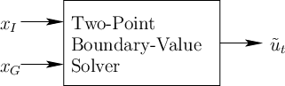Under the first alternative, the BVP solver can be considered as a black box, as shown in Figure 14.10, that efficiently connects ${x_{I}}$ to ${x_{G}}$ in the absence of obstacles. In the case of the Piano Mover's Problem, this was obtained by moving along the shortest path in ${\cal C}$. For many of the wheeled vehicle systems from Section 13.1.2, steering methods exist that could serve as an efficient BVP solver; see Section 15.5. Efficient techniques also exist for linear systems and are covered in Section 15.2.2.

If the BVP is efficiently solved, then virtually any sampling-based planning algorithm from Chapter 5 can be adapted to the case of differential constraints. This is achieved by using the module in Figure 14.10 as the LPM. For example, a sampling-based roadmap can use the computed solution in the place of the shortest path through ${\cal C}$. If the BVP solver is not efficient enough, then this approach becomes impractical because it must typically be used thousands of times to build a roadmap. The existence of an efficient module as shown in Figure 14.10 magically eliminates most of the complications associated with planning under differential constraints. The only remaining concern is that the solutions provided by the BVP solver could be quite long in comparison to the shortest path in the absence of differential constraints (for example, how far must the Dubins car travel to move slightly backward?).

Under the second alternative, it is assumed that solving the BVP is very costly. The planning method in this case should avoid solving BVPs whenever possible. Some planning algorithms may only require an LPM that approximately reaches intermediate goal states, which is simpler for some systems. Other planning algorithms may not require the LPM to make any kind of connection. The LPM may return a motion primitive that appears to make some progress in the search but is not designed to connect to a prescribed state. This usually involves incremental planning methods, which are covered in Section 14.4 and extends the methods of Sections 5.4 and 5.5 to handle differential constraints.