13.4.3.1 Incorporating velocity constraints

The Lagrangian formulation of Section 13.4.1 can be extended to allow additional constraints placed on $q$ and ${\dot q}$. This is very powerful for developing state transition equations for robots that have closed kinematic chains or wheeled bodies. If there are closed chains, then the configurations may be restricted to lie in a subset of ${\cal C}$. If a parameterization of the solution set is possible, then ${\cal C}$ can be redefined over the reduced C-space. This is usually not possible, however, because such a parametrization is difficult to obtain, as mentioned in Section 4.4. If there are wheels or other contact-based constraints, such as those in Section 13.1.3, then extra constraints on $q$ and ${\dot q}$ exist. Dynamics can be incorporated into the models of Section 13.1 by extending the Euler-Lagrange equation.

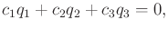
The coming method will be based on Lagrange multipliers. Recall from standard calculus that to optimize a function $h$ defined over ${\mathbb{R}}^n$, subject to an implicit constraint $g(x) = 0$, it is sufficient to consider only the extrema of

$$h(x) + \lambda g(x) ,$$ (13.162)

in which $\lambda \in {\mathbb{R}}$ represents a Lagrange multiplier [508]. The extrema are found by solving

$$\nabla h(x) + \lambda \nabla g(x) = 0 ,$$ (13.163)

which expresses $n$ equations of the form

$$\frac{\partial h}{\partial x_i} + \lambda \frac{\partial g}{\partial x_i} = 0 .$$ (13.164)

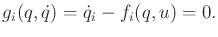
The same principle applies for handling velocity constraints on ${\cal C}$.

Suppose that there are velocity constraints on ${\cal C}$ as considered in Section 13.1. Consider implicit constraints, in which there are $k$ equations of the form $g_i(q,{\dot q}) = 0$ for $i$ from $1$ to $k$. Parametric constraints can be handled as a special case of implicit constraints by writing

$$g_i(q,{\dot q}) = {\dot q}_i - f_i(q,u) = 0.$$ (13.165)

For any constraints that contain actions $u$, no extra difficulties arise. Each $u_i$ is treated as a constant in the following analysis. Therefore, action variables will not be explicitly named in the expressions.

As before, assume time-invariant dynamics (see [789] for the time-varying case). Starting with $L(q,{\dot q})$ defined using (13.130), let the new criterion be

$$L_c(q,{\dot q},\lambda) = L(q,{\dot q}) + \sum_{i=1}^k \lambda_i g_i(q,{\dot q}) .$$ (13.166)

A functional $\Phi_c$ is defined by substituting $L_c$ for $L$ in (13.114).

The extremals of $\Phi_c$ are given by $n$ equations,

$$\frac{d}{dt} \frac{\partial L_c}{\partial {\dot q}_i} - \frac{\partial L_c}{\partial q_i} = 0 ,$$ (13.167)

and $k$ equations,

$$\frac{d}{dt} \frac{\partial L_c}{\partial {\dot \lambda}_i} - \frac{\partial L_c}{\partial \lambda_i} = 0 .$$ (13.168)

The justification for this is the same as for (13.124), except now $\lambda$ is included. The equations of (13.168) are equivalent to the constraints $g_i(q,{\dot q}) = 0$. The first term of each is zero because ${\dot \lambda}$ does not appear in the constraints, which reduces them to

$$\frac{\partial L_c}{\partial \lambda_i} = 0 .$$ (13.169)

This already follows from the constraints on extremals of $L$ and the constraints $g_i(q,{\dot q}) = 0$. In (13.167), there are $n$ equations in $n + k$ unknowns. The $k$ Lagrange multipliers can be eliminated by using the $k$ constraints $g_i(q,{\dot q}) = 0$. This corresponds to Lagrange multiplier elimination in standard constrained optimization [508].

The expressions in (13.167) and the constraints $g_i(q,{\dot q})$ may be quite complicated, which makes the determination of a state transition equation challenging. General forms are given in Section 3.8 of [789]. An important special case will be considered here. Suppose that the constraints are Pfaffian,

$$g_i(q,{\dot q}) = \sum_{j=1}^n g_{ij}(q) {\dot q}_j = 0 ,$$ (13.170)

as introduced in Section 13.1. This includes the nonholonomic velocity constraints due to wheeled vehicles, which were presented in Section 13.1.2. Furthermore, this includes the special case of constraints of the form $g_i(q) = 0$, which models closed kinematic chains. Such constraints can be differentiated with respect to time to obtain

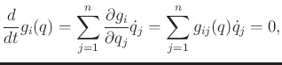$$\frac{d}{dt} g_i(q) = \sum_{j=1}^n \frac{\partial g_i}{\partial q_j} {\dot q}_j = \sum_{j=1}^n g_{ij}(q) {\dot q}_j = 0 ,$$ (13.171)

which is in the Pfaffian form. This enables the dynamics of closed chains, considered in Section 4.4, to be expressed without even having a parametrization of the subset of ${\cal C}$ that satisfies the closure constraints. Starting in implicit form, differentiation is required to convert them into the Pfaffian form.

For the important case of Pfaffian constraints, (13.167) simplifies to

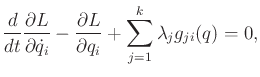$$\frac{d}{dt} \frac{\partial L}{\partial {\dot q}_i} - \frac{\partial L}{\partial q_i} + \sum_{j=1}^k \lambda_j g_{ji}(q) = 0 ,$$ (13.172)

The Pfaffian constraints can be used to eliminate the Lagrange multipliers, if desired. Note that $g_{ji}$ represents the $i$th term of the $j$th Pfaffian constraint. An action variable $u_i$ can be placed on the right side of each constraint, if desired.

Equation (13.172) often appears instead as

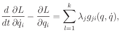$$\frac{d}{dt} \frac{\partial L}{\partial {\dot q}_i} - \frac{\partial L}{\partial q_i} = \sum_{l=1}^k \lambda_j g_{ji}(q,{\dot q}) ,$$ (13.173)

which is an alternative but equivalent expression of constraints because the Lagrange multipliers can be negated without affecting the existence of extremals. In this case, a nice interpretation due to D'Alembert can be given. Expressions that appear on the right of (13.173) can be considered as actions, as mentioned in Section 13.4.1. As stated previously, such actions are called generalized forces in mechanics. The principle of virtual work is obtained by integrating the reaction forces needed to maintain the constraints. These reaction forces are precisely given on the right side of (13.173). Due to the cancellation of forces, no true work is done by the constraints (if there is no friction).

Example 13..14 (A Particle on a Sphere)   Suppose that a particle travels on a unit sphere without friction or gravity. Let $(q_1,q_2,q_3) \in {\mathbb{R}}^3$ denote the position of the point. The Lagrangian function is the kinetic energy,

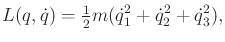$$L(q,{\dot q}) = \begin{matrix}\frac{1}{2} \end{matrix} m ({\dot q}_1^2 + {\dot q}_2^2 + {\dot q}_3^2) ,$$ (13.174)

in which $m$ is the particle mass. For simplicity, assume that $m=2$.

The constraint that the particle must travel on a sphere yields

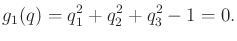$$g_1(q) = q_1^2 + q_2^2 + q_3^2 - 1 = 0 .$$ (13.175)

This can be put into Pfaffian form by time differentiation to obtain

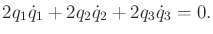$$2 q_1 {\dot q}_1 + 2 q_2 {\dot q}_2 + 2 q_3 {\dot q}_3 = 0 .$$ (13.176)

Since $k=1$, there is a single Lagrange multiplier $\lambda_1$. Applying (13.172) yields three equations,

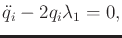$${\ddot q}_i - 2 q_i \lambda_1 = 0 ,$$ (13.177)

for $i$ from $1$ to $3$. The generic form of the solution is

$$c_1 q_1 + c_2 q_2 + c_3 q_3 = 0 ,$$ (13.178)

in which the $c_i$ are real-valued constants that can be determined from the initial position of the particle. This represents the equation of a plane through the origin. The intersection of the plane with the sphere is a great circle. This implies that the particle moves between two points by traveling along the great circle. These are the shortest paths (geodesics) on the sphere. $\blacksquare$

The general forms in Section 13.4.2 can be extended to the constrained case. For example, (13.142) generalizes to

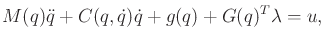$$M(q) {\ddot q}+ C(q,{\dot q}){\dot q}+ g(q) + G(q)^T \lambda = u ,$$ (13.179)

in which $G$ is a $n \times k$ matrix that represents all of the $g_{ji}$ Pfaffian coefficients. In this case, the Lagrange multipliers can be computed as [725]

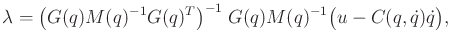$$\lambda = \big( G(q)M(q)^{-1}G(q)^T \big)^{-1}\;G(q)M(q)^{-1}\big(u - C(q,{\dot q}){\dot q}\big),$$ (13.180)

assuming $G$ is time-invariant.

The phase transition equation can be determined in the usual way by performing the required differentiations, defining the $2n$ phase variables, and solving for ${\dot x}$. The result generalizes (13.148).