13.4.2.1 Conversion to a phase transition equation

The final step is to convert the equations into phase space form. A $2n$-dimensional phase vector is introduced as $x = (q,{\dot q})$. The task is to obtain ${\dot x}= f(x,u)$, which represents $2n$ scalar equations. The first $n$ equations are ${\dot x}_i = x_{n+i}$ for $i$ from $1$ to $n$. The final $n$ equations are obtained by solving for ${\ddot q}$.

Suppose that the general form in (13.142) is used. Solving for ${\ddot q}$ yields

$${\ddot q}= M(q)^{-1}(u - C(q,{\dot q}){\dot q}- g(q)) .$$ (13.148)

The phase variables are then substituted in a straightforward manner. Each ${\ddot q}_i$ for $i$ from $1$ to $n$ becomes ${\dot x}_{n+i}$, and $M(q)$, $C(q,{\dot q})$, and $g(q)$ are expressed in terms of $x$. This completes the specification of the phase transition equation.

Example 13..13 (Two-Link Manipulator)  

Figure 13.13: Parameter values for a two-link robot with two revolute joints.

Figure 13.13 shows a two-link manipulator for which there are two revolute joints and two links, ${\cal A}_1$ and ${\cal A}_2$. Hence, ${\cal C} = {\mathbb{S}}^1 \times {\mathbb{S}}^1$. Let $q = (\theta_1,\theta_2)$ denote a configuration. Each of the two joints is controlled by a motor that applies a torque $u_i$. Let $u_1$ apply to the base, and let $u_2$ apply to the joint between ${\cal A}_1$ and ${\cal A}_2$. Let $d_1$ be the link length of ${\cal A}_1$. Let $\ell_i$ be the distance from the ${\cal A}_i$ origin to its center of mass. For each ${\cal A}_i$, let $m_i$ and $I_i$ be its mass and moment of inertia, respectively.

The kinetic energy of ${\cal A}_1$ is

$$K_1({\dot q}) = \begin{matrix}\frac{1}{2} \end{matrix} m_1 \ell_1... ...ot \theta}_1^2 + \begin{matrix}\frac{1}{2} \end{matrix} I_1 {\dot \theta}_1^2 ,$$ (13.149)

and the potential energy of ${\cal A}_1$ is

$$V_1(q) = m_1 g \ell_1 \sin\theta_1 .$$ (13.150)

The kinetic energy of ${\cal A}_2$ is

$$K_2({\dot q}) = \begin{matrix}\frac{1}{2} \end{matrix} p \cdot p ... ...gin{matrix}\frac{1}{2} \end{matrix} I_2 ({\dot \theta}_1 + {\dot \theta}_2)^2 ,$$ (13.151)

in which $p$ denotes the position of the center of mass of ${\cal A}_1$ and is given from (3.53) as

$$\begin{split}p_1 = d_1 \cos\theta_1 + \ell_2 \cos\theta_2 \\ p_2 = d_1 \sin\theta_1 + \ell_2 \sin\theta_2 . \end{split}$$ (13.152)

The potential energy of ${\cal A}_2$ is

$$V_2(q) = m_2 g (d_1 \sin\theta_1 + \ell_2 \sin\theta_2) .$$ (13.153)

At this point, the Lagrangian function can be formed as

$$L(q,{\dot q}) = K_1({\dot \theta}_1) + K_2({\dot \theta}_1,{\dot \theta}_2) - V_1(\theta_1) - V_2(\theta_1,\theta_2)$$ (13.154)

and inserted into (13.118) to obtain the differential constraints in implicit form, expressed in terms of ${\ddot q}$, ${\dot q}$, and $q$. Conversion to the phase space is performed by solving the implicit constraints for ${\ddot q}$ and assigning $x = (q,{\dot q})$, in which $x$ is a four-dimensional phase vector.

Rather than performing the computations directly using (13.118), the constraints can be directly determined using (13.140). The terms are

$$M(q) = \begin{pmatrix}m_{11} & m_{12} \\ m_{21} & m_{22} \end{pmatrix} ,$$ (13.155)

in which

$$\begin{split}m_{11} & = I_1 + m_1 \ell_1^2 + I_2 + m_2(d_1^2 ... ..._2 \cos\theta_2) \\ m_{22} & = I_2 + m_2 \ell_2^2 , \end{split}$$ (13.156)

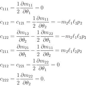
and

$$\begin{split}c_{111} & = \frac{1}{2} \frac{\partial m_{11}}{\... ...}{2} \frac{\partial m_{22}}{\partial\theta_2} = 0 . \end{split}$$ (13.157)

The final term is defined as

$$\begin{split}g_1 & = (m_1 \ell_1 + m_2 d_1) g p_1 + m_1 \ell_2 p_2 \\ g_2 & = m_2 \ell_2 g p_2 . \end{split}$$ (13.158)

The dynamics can alternatively be expressed using $M(q)$, $C(q,{\dot q})$, and $g(q)$ in (13.142). The Coriolis matrix is defined using (13.143) to obtain

$$C(q,{\dot q}) = -m_2 \ell_1 \ell_2 p_2 \begin{pmatrix}{\dot \theta}_2 & {\dot \theta}_1 + {\dot \theta}_2 \\ {\dot \theta}_1 & 0 \end{pmatrix} ,$$ (13.159)

in which $p_2$ is defined in (13.152) and is a function of $q$. For convenience, let

$$r = m_2 \ell_1 \ell_2 p_2 .$$ (13.160)

The resulting expression, which is now a special form of (13.142), is

$$\begin{split}m_{11} {\ddot \theta}_1 + m_{12} {\ddot \theta}_... ... \theta}_2 + r {\dot \theta}_1^2 + g_2(q) & = u_2 . \end{split}$$ (13.161)

The phase transition equation is obtained by letting $x = (\theta_1,\theta_2,{\dot \theta}_1,{\dot \theta}_2)$ and substituting the state variables into (13.161). The variables ${\ddot \theta}_1$ and ${\ddot \theta}_2$ become ${\dot x}_3$ and ${\dot x}_4$, respectively. The equations must be solved for ${\dot x}_3$ and ${\dot x}_4$. An extension of this model to motors that have gear ratios and nonnegligible mass appears in [856]. $\blacksquare$

The example provided here barely scratches the surface on the possible systems that can be elegantly modeled. Many robotics texts cover cases in which there are more links, different kinds of joints, and frictional forces [366,725,856,907,994].

The phase transition equation for chains of bodies could alternatively be derived using the Newton-Euler formulation of mechanics. Even though the Lagrangian form is more elegant, the Newton-Euler equations, when expressed recursively, are far more efficient for simulations of multibody dynamical systems [366,863,994].