
Next: 11.3.2 Nondeterministic Finite Automata Up: 11.3 Examples for Discrete Previous: 11.3 Examples for Discrete
First, we consider a simple example that uses the sign sensor of Example 11.3.
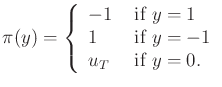
The general expression for a history I-state at stage ![]() is
is
| (11.42) |
The solution can even be implemented with sensor feedback because the
action depends only on the current sensor value. Let
![]() be defined as
be defined as
 |
(11.43) |
The next example provides a simple illustration of solving a problem without ever knowing the current state. This leads to the goal recognizability problem [659] (see Section 12.5.1).
The problem shown in Figure 11.7 serves two purposes.
First, it is an example of sensorless planning[321,394], which means that there are no observations (see
Sections 11.5.4 and 12.5.2). This is an
interesting class of problems because it appears that no information
can be gained regarding the state. Contrary to intuition, it turns
out for this example and many others that plans can be designed that
estimate the state. The second purpose is to illustrate how the
I-space can be dramatically collapsed using the I-map concepts of
Section 11.2.1. The standard nondeterministic I-space for
this example contains ![]() I-states, but it can be mapped to a
much smaller derived I-space that contains only a few elements.
I-states, but it can be mapped to a
much smaller derived I-space that contains only a few elements.
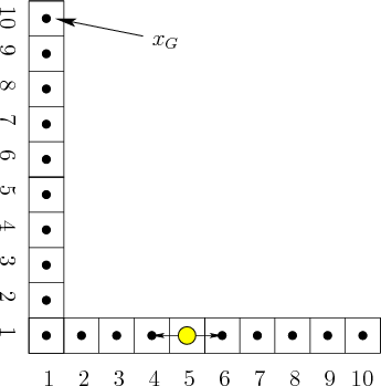 |
There are no sensor observations for this problem. However, nature interferes with the state transitions, which leads to a form of nondeterministic uncertainty. If an action is applied that tries to take one step, nature may cause two or three steps to be taken. This can be modeled as follows. Let
| (11.44) |
Since there are no sensor observations, the history I-state at stage
![]() is
is
| (11.45) |
With perfect information, this would be trivial; however, without
sensors the uncertainty may grow very quickly. For example, after
applying the action
![]() from the initial state, the
nondeterministic I-state becomes
from the initial state, the
nondeterministic I-state becomes
![]() . After
. After
![]() it becomes
it becomes
![]() . A nice feature of this
problem, however, is that uncertainty can be reduced without sensing.
Suppose that for
. A nice feature of this
problem, however, is that uncertainty can be reduced without sensing.
Suppose that for ![]() stages, we repeatedly apply
stages, we repeatedly apply
![]() .
What is the resulting I-state? As the corner state is approached, the
uncertainty is reduced because the state cannot be further changed by
nature. It is known that each action,
.
What is the resulting I-state? As the corner state is approached, the
uncertainty is reduced because the state cannot be further changed by
nature. It is known that each action,
![]() , decreases the
, decreases the
![]() coordinate by at least one each time. Therefore, after nine or
more stages, it is known that
coordinate by at least one each time. Therefore, after nine or
more stages, it is known that
![]() . Once this is
known, then the action
. Once this is
known, then the action ![]() can be applied. This will again
increase uncertainty as the state moves through the set of left
states. If
can be applied. This will again
increase uncertainty as the state moves through the set of left
states. If ![]() is applied nine or more times, then it is known for
certain that
is applied nine or more times, then it is known for
certain that
![]() , which is the required goal state.
, which is the required goal state.
A successful plan has now been obtained: 1) Apply ![]() for nine
stages, 2) then apply
for nine
stages, 2) then apply ![]() for nine stages. This plan could be
defined over
for nine stages. This plan could be
defined over
![]() ; however, it is simpler to use the I-map
; however, it is simpler to use the I-map
![]() from Example 11.12 to define a plan as
from Example 11.12 to define a plan as
![]() . For
. For ![]() such that
such that
![]() ,
,
![]() . For
. For ![]() such that
such that
![]() ,
,
![]() . For
. For ![]() ,
,
![]() . Note that the
plan works even if the initial condition is any subset of
. Note that the
plan works even if the initial condition is any subset of ![]() . From
this point onward, assume that any subset may be given as the initial
condition.
. From
this point onward, assume that any subset may be given as the initial
condition.
Some alternative plans will now be considered by making other derived
I-spaces from
![]() . Let
. Let
![]() be an I-map from
be an I-map from
![]() to a set
to a set
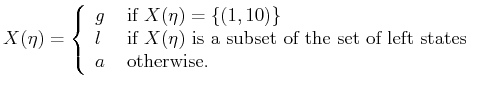
![]() of three derived I-states. Let
of three derived I-states. Let
![]() , in which
, in which ![]() denotes ``goal,''
denotes ``goal,'' ![]() denotes ``left,'' and
denotes ``left,'' and
![]() denotes ``any.'' The I-map,
denotes ``any.'' The I-map,
![]() , is
, is
 |
(11.46) |
To address this problem, consider a new I-map,
![]() , which is sufficient. There are
, which is sufficient. There are ![]() derived
I-states, which include
derived
I-states, which include ![]() as defined previously,
as defined previously, ![]() for
for
![]() , and
, and ![]() for
for
![]() . The I-map is defined as
. The I-map is defined as
![]() if
if
![]() . Otherwise,
. Otherwise,
![]() for the smallest value of
for the smallest value of ![]() such that
such that
![]() is a subset of
is a subset of
![]() . If there is no
such value for
. If there is no
such value for ![]() , then
, then
![]() , for the smallest
value of
, for the smallest
value of ![]() such that
such that ![]() is a subset of
is a subset of
![]() . Now the plan is defined
as
. Now the plan is defined
as
![]() ,
,
![]() , and
, and
![]() . Although the plan is larger, the robot does not need to
represent the full nondeterministic I-state during execution. The
correct transitions occur. For example, if
. Although the plan is larger, the robot does not need to
represent the full nondeterministic I-state during execution. The
correct transitions occur. For example, if
![]() is applied
at
is applied
at ![]() , then
, then ![]() is obtained. If
is obtained. If
![]() is applied at
is applied at
![]() , then
, then ![]() is obtained. From there,
is obtained. From there, ![]() is applied to
yield
is applied to
yield ![]() . These actions can be repeated until eventually
. These actions can be repeated until eventually ![]() and
and
![]() are reached. The resulting plan, however, is not an improvement
over the original open-loop one.
are reached. The resulting plan, however, is not an improvement
over the original open-loop one.
![]()
Steven M LaValle 2020-08-14