General optimality criteria

It is difficult to even define optimality for more general C-spaces. What does it mean to have a shortest path in $SE(2)$ or $SE(3)$? Consider the case of a planar, rigid robot that can translate and rotate. One path could minimize the amount of rotation whereas another tries to minimize the amount of translation. Without more information, there is no clear preference. Ulam's distance is one possibility, which is to minimize the distance traveled by $k$ fixed points [474]. In Chapter 13, differential models will be introduced, which lead to meaningful definitions of optimality. For example, the shortest paths for a slow-moving car are shown in Section 15.3; these require a precise specification of the constraints on the motion of the car (it is more costly to move a car sideways than forward).

This section formulates some optimal motion planning problems, to provide a smooth transition into the later concepts. Up until now, actions were used in Chapter 2 for discrete planning problems, but they were successfully avoided for basic motion planning by directly describing paths that map into ${\cal C}_{free}$. It will be convenient to use them once again. Recall that they were convenient for defining costs and optimal planning in Section 2.3.

To avoid for now the complications of differential equations, consider making an approximate model of motion planning in which every path must be composed of a sequence of shortest-path segments in ${\cal C}_{free}$. Most often these are line segments; however, for the case of $SO(3)$, circular arcs obtained by spherical linear interpolation may be preferable. Consider extending Formulation 2.3 from Section 2.3.2 to the problem of motion planning.

Let the C-space ${\cal C}$ be embedded in ${\mathbb{R}}^m$ (i.e., ${\cal C}\subset {\mathbb{R}}^m$). An action will be defined shortly as an $m$-dimensional vector. Given a scaling constant $\epsilon$ and a configuration $q$, an action $u$ produces a new configuration, $q^\prime = q + \epsilon u$. This can be considered as a configuration transition equation, $q^\prime = f(q,u)$. The path segment represented by the action $u$ is the shortest path (usually a line segment) between $q$ and $q^\prime$. Following Section 2.3, let $\pi _K$ denote a $K$-step plan, which is a sequence $(u_1$, $u_2$, $\ldots$, $u_K)$ of $K$ actions. Note that if $\pi _K$ and ${q_{I}}$ are given, then a sequence of states, $q_1$, $q_2$, $\ldots$, $q_{K+1}$, can be derived using $f$. Initially, $q_1 = {q_{I}}$, and each following state is obtained by $q_{k+1} = f(q_k,u_k)$. From this a path, $\tau: [0,1] \rightarrow {\cal C}$, can be derived.

An approximate optimal planning problem is formalized as follows:

Formulation 7..4 (Approximate Optimal Motion Planning)  

1. The following components are defined the same as in Formulation 4.1: ${\cal W}$, ${\cal O}$, ${\cal A}$, ${\cal C}$, ${\cal C}_{obs}$, ${\cal C}_{free}$, and ${q_{I}}$. It is assumed that ${\cal C}$ is an $n$-dimensional manifold.
2. For each $q \in {\cal C}$, a possibly infinite action space, $U(q)$. Each $u \in U$ is an $n$-dimensional vector.
3. A positive constant $\epsilon > 0$ called the step size.
4. A set of stages, each denoted by $k$, which begins at $k=1$ and continues indefinitely. Each stage is indicated by a subscript, to obtain $q_k$ and $u_k$.
5. A configuration transition function $f(q,u) = q + \epsilon u$ in which $q+\epsilon u$ is computed by vector addition on ${\mathbb{R}}^m$.
6. Instead of a goal state, a goal region $X_G$ is defined.
7. Let $L$ denote a real-valued cost functional, which is applied to a $K$-step plan, $\pi _K$. This means that the sequence $(u_1,\ldots,u_K)$ of actions and the sequence $(q_1,\ldots,q_{K+1})$ of configurations may appear in an expression of $L$. Let $F = K+1$. The cost functional is

   $$L(\pi _K) = \sum_{k=1}^K l(q_k,u_k) + l_F(q_F) .$$ (7.26)

   
   
   The final term $l_F(q_F)$ is outside of the sum and is defined as $l_F(q_F) = 0$ if $q_F \in X_G$ and $l_F(q_F) = \infty$ otherwise. As in Formulation 2.3, $K$ is not necessarily a constant.
8. Each $U(q)$ contains the special termination action $u_T$, which behaves the same way as in Formulation 2.3. If $u_T$ is applied to $q_k$ at stage $k$, then the action is repeatedly applied forever, the configuration remains in $q_k$ forever, and no more cost accumulates.

The task is to compute a sequence of actions that optimizes (7.26). Formulation 7.4 can be used to define a variety of optimal planning problems. The parameter $\epsilon$ can be considered as the resolution of the approximation. In many formulations it can be interpreted as a time step, $\epsilon = \Delta t$; however, note that no explicit time reference is necessary because the problem only requires constructing a path through ${\cal C}_{free}$. As $\epsilon$ approaches zero, the formulation approaches an exact optimal planning problem. To properly express the exact problem, differential equations are needed. This is deferred until Part IV.

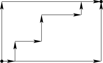
Figure 7.40: Under the Manhattan ($L_1$) motion model, all monotonic paths that follow the grid directions have equivalent length.

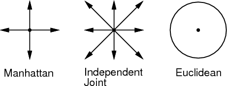
Figure 7.41: Depictions of the action sets, $U(q)$, for Examples 7.4, 7.5, and 7.6.

Example 7..4 (Manhattan Motion Model)   Suppose that in addition to $u_T$, the action set $U(q)$ contains $2n$ vectors in which only one component is nonzero and must take the value $1$ or $-1$. For example, if ${\cal C}= {\mathbb{R}}^2$, then

$$U(q) = \{(1,0),(-1,0),(0,-1),(0,1),u_T\}.$$ (7.27)

When used in the configuration transition equation, this set of actions produces ``up,'' ``down,'' ``left,'' and ``right'' motions and a ``terminate'' command. This produces a topological graph according to the 1-neighborhood model, (5.37), which was given in Section 5.4.2. The action set for this example and the following two examples are shown in Figure 7.41 for comparison. The cost term $l(q_k,u_k)$ is defined to be $1$ for all $q_k \in {\cal C}_{free}$ and $u_k$. If $q_k \in {\cal C}_{obs}$, then $l(q_k,u_k) = \infty$. Note that the set of configurations reachable by these actions lies on a grid, in which the spacing between $1$-neighbors is $\epsilon$. This corresponds to a convenient special case in which time discretization (implemented by $\epsilon$) leads to a regular space discretization. Consider Figure 7.40. It is impossible to take a shorter path along a diagonal because the actions do not allow it. Therefore, all monotonic paths along the grid produce the same costs.

Optimal paths can be obtained by simply applying the dynamic programming algorithms of Chapter 2. This example provides a nice unification of concepts from Section 2.2, which introduced grid search, and Section 5.4.2, which explained how to adapt search methods to motion planning. In the current setting, only algorithms that produce optimal solutions on the corresponding graph are acceptable.

This form of optimization might not seem relevant because it does not represent the Euclidean shortest-path problem for ${\mathbb{R}}^2$. The next model adds more actions, and does correspond to an important class of optimization problems in robotics. $\blacksquare$

Example 7..5 (Independent-Joint Motion Model)   Now suppose that $U(q)$ includes $u_T$ and the set of all $3^n$ vectors for which every element is either $-1$, 0, or $1$. Under this model, a path can be taken along any diagonal. This still does not change the fact that all reachable configurations lie on a grid. Therefore, the standard grid algorithms can be applied once again. The difference is that now there are $3^n-1$ edges emanating from every vertex, as opposed to $2n$ in Example 7.4. This model is appropriate for robots that are constructed from a collection of links attached by revolute joints. If each joint is operated independently, then it makes sense that each joint could be moved either forward, backward, or held stationary. This corresponds exactly to the actions. However, this model cannot nicely approximate Euclidean shortest paths; this motivates the next example. $\blacksquare$

Example 7..6 (Euclidean Motion Model)   To approximate Euclidean shortest paths, let $U(q) = {\mathbb{S}}^{n-1} \cup \{u_T\}$, in which ${\mathbb{S}}^{n-1}$ is the $m$-dimensional unit sphere centered at the origin of ${\mathbb{R}}^n$. This means that in $k$ stages, any piecewise-linear path in which each segment has length $\epsilon$ can be formed by a sequence of inputs. Therefore, the set of reachable states is no longer confined to a grid. Consider taking $\epsilon = 1$, and pick any point, such as $(\pi,\pi) \in {\mathbb{R}}^2$. How close can you come to this point? It turns out that the set of points reachable with this model is dense in ${\mathbb{R}}^n$ if obstacles are neglected. This means that we can come arbitrarily close to any point in ${\mathbb{R}}^n$. Therefore, a finite grid cannot be used to represent the problem. Approximate solutions can still be obtained by numerically computing an optimal cost-to-go function over ${\cal C}$. This approach is presented in Section 8.5.2.

One additional issue for this problem is the precision defined for the goal. If the goal region is very small relative to $\epsilon$, then complicated paths may have to be selected to arrive precisely at the goal. $\blacksquare$

Example 7..7 (Weighted-Region Problem)   In outdoor and planetary navigation applications, it does not make sense to define obstacles in the crisp way that has been used so far. For each patch of terrain, it is more convenient to associate a cost that indicates the estimated difficulty of its traversal. This is sometimes considered as a ``grayscale'' model of obstacles. The model can be easily captured in the cost term $l(q_k,u_k)$. The action spaces can be borrowed from Examples 7.4 or 7.5. Stentz's algorithm [913], which is introduced in Section 12.3.2, generates optimal navigation plans for this problem, even assuming that the terrain is initially unknown. Theoretical bounds for optimal weighted-region planning problems are given in [709,710]. An approximation algorithm appears in [820]. $\blacksquare$