15.4.2.2 Distributions

A distribution^15.8 expresses a set of vector fields on a smooth manifold. Suppose that a driftless control-affine system (15.53) is given. Recall the vector space definition from Section 8.3.1 or from linear algebra. Also recall that a state transition equation can be interpreted as a vector field if the actions are fixed and as a vector space if the state is instead fixed. For $U = {\mathbb{R}}^m$ and a fixed $x \in X$, the state transition equation defines a vector space in which each $h_i$ evaluated at $x$ is a basis vector and each $u_i$ is a coefficient. 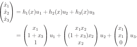For example, in (15.54), the vector fields $h_1$ and $h_2$ evaluated at $q = (0,0,0)$ become $[1 \;\; 0 \;\; 0]^T$ and $[0 \;\; 0 \;\; 1]^T$, respectively. These serve as the basis vectors. By selecting values of $u \in {\mathbb{R}}^2$, a 2D vector space results. Any vector of the form $[a \; \; 0 \;\; b]^T$ can be represented by setting $u_1 = a$ and $u_2 = b$. More generally, let ${\triangle}(x)$ denote the vector space obtained in this way for any $x \in X$.

The dimension of a vector space is the number of independent basis vectors. Therefore, the dimension of ${\triangle}(x)$ is the rank of $H(x)$ from (15.56) when evaluated at the particular $x \in X$. Now consider defining ${\triangle}(x)$ for every $x \in X$. This yields a parameterized family of vector spaces, one for each $x \in X$. The result could just as well be interpreted as a parameterized family of vector fields. For example, consider actions for $i$ from $1$ to $m$ of the form $u_i = 1$ and $u_j = 0$ for all $i \not = j$. If the action is held constant over all $x \in X$, then it selects a single vector field $h_i$ from the collection of $m$ vector fields:

$${\dot x}= h_i(x) .$$ (15.63)

Using constant actions, an $m$-dimensional vector space can be defined in which each vector field $h_i$ is a basis vector (assuming the $h_i$ are linearly independent), and the $u_i \in {\mathbb{R}}$ are the coefficients:

$$u_1 h_1(x) + u_2 h_2(x) + \cdots + u_m h_m(x) .$$ (15.64)

This idea can be generalized to allow the $u_i$ to vary over $X$. Thus, rather than having $u$ constant, it can be interpreted as a feedback plan $\pi : X \rightarrow U$, in which the action at $x$ is given by $u = \pi (x)$. The set of all vector fields that can be obtained as

$$\pi _1(x) h_1(x) + \pi _2(x) h_2(x) + \cdots + \pi _m(x) h_m(x)$$ (15.65)

is called the distribution of the set $\{h_1,\ldots,h_m\}$ of vector fields and is denoted as ${\triangle }$. If ${\triangle }$ is obtained from an control-affine system, then ${\triangle }$ is called the system distribution. The resulting set of vector fields is not quite a vector space because the nonzero coefficients $\pi_i$ do not necessarily have a multiplicative inverse. This is required for the coefficients of a vector field and was satisfied by using ${\mathbb{R}}$ in the case of constant actions. A distribution is instead considered algebraically as a module [469]. In most circumstances, it is helpful to imagine it as a vector space (just do not try to invert the coefficients!). Since a distribution is almost a vector space, the $\operatorname{span}$ notation from linear algebra is often used to define it:

$${\triangle}= \operatorname{span}\{h_1,h_2,\ldots,h_m\} .$$ (15.66)

Furthermore, it is actually a vector space with respect to constant actions $u \in {\mathbb{R}}^m$. Note that for each fixed $x \in X$, the vector space ${\triangle}(x)$ is obtained, as defined earlier. A vector field $f$ is said to belong to a distribution ${\triangle }$ if it can be expressed using (15.65). If for all $x \in X$, the dimension of ${\triangle}(x)$ is $m$, then ${\triangle }$ is called a nonsingular distribution (or regular distribution). Otherwise, ${\triangle }$ is called a singular distribution, and the points $x \in X$ for which the dimension of ${\triangle}(x)$ is less than $m$ are called singular points. If the dimension of ${\triangle}(x)$ is a constant $c$ over all $x \in X$, then $c$ is called the dimension of the distribution and is denoted by $\dim({\triangle})$. If the vector fields are smooth, and if $\pi$ is restricted to be smooth, then a smooth distribution is obtained, which is a subset of the original distribution.

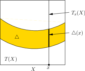
Figure 15.15: The distribution ${\triangle }$ can be imagined as a slice of the tangent bundle $T(X)$. It restricts the tangent space at every $x \in X$.

As depicted in Figure 15.15, a nice interpretation of the distribution can be given in terms of the tangent bundle of a smooth manifold. The tangent bundle was defined for $X = {\mathbb{R}}^n$ in (8.9) and generalizes to any smooth manifold $X$ to obtain

$$T(X) = \bigcup_{x \in X} T_x(X) .$$ (15.67)

The tangent bundle is a $2n$-dimensional manifold in which $n$ is the dimension of $X$. A phase space for which $x = (q,{\dot q})$ is actually $T({\cal C})$. In the current setting, each element of $T(X)$ yields a state and a velocity, $(x,{\dot x})$. Which pairs are possible for a driftless control-affine system? Each ${\triangle}(x)$ indicates the set of possible ${\dot x}$ values for a fixed $x$. The point $x$ is sometimes called the base and ${\triangle}(x)$ is called the fiber over $x$ in $T(X)$. The distribution ${\triangle }$ simply specifies a subset of $T_x(X)$ for every $x \in X$. For a vector field $f$ to belong to ${\triangle }$, it must satisfy $f(x) \in {\triangle}(x)$ for all $x \in X$. This is just a restriction to a subset of $T(X)$. If $m = n$ and the system vector fields are independent, then any vector field is allowed. In this case, ${\triangle }$ includes any vector field that can be constructed from the vectors in $T(X)$.

Example 15..7 (The Distribution for the Differential Drive)   The system in (15.54) yields a two-dimensional distribution:

$${\triangle}= \operatorname{span}\{ [\cos\theta \;\; \sin\theta \;\; 0]^T, \; [0 \;\; 0 \;\; 1]^T\} .$$ (15.68)

The distribution is nonsingular because for any $(x,y,\theta)$ in the coordinate neighborhood, the resulting vector space ${\triangle}(x,y,\theta)$ is two-dimensional. $\blacksquare$

Example 15..8 (A Singular Distribution)   Consider the following system, which is given in [478]:

$$\begin{split}\begin{pmatrix}{\dot x}_1 \\ {\dot x}_2 \\ {\dot... ...egin{pmatrix}x_1 \\ x_1 \\ 0 \\ \end{pmatrix} u_3 . \end{split}$$ (15.69)

The distribution is

$${\triangle}= \operatorname{span}\{h_1,h_2,h_3\}.$$ (15.70)

The first issue is that for any $x \in {\mathbb{R}}^3$, $h_2(x) = h_1(x) x_2$, which implies that the vector fields are linearly dependent over all of ${\mathbb{R}}^3$. Hence, this distribution is singular because $m = 3$ and the dimension of $\Delta(x)$ is $2$ if $x_1 \not = 0$. If $x_1 = 0$, then the dimension of $\Delta(x)$ drops to $1$. The dimension of ${\triangle }$ is not defined because the dimension of $\Delta(x)$ depends on $x$. $\blacksquare$

A distribution can alternatively be defined directly from Pfaffian constraints. Each $g_i(x) = 0$ is called an annihilator because enforcing the constraint eliminates many vector fields from consideration. At each $x \in X$, ${\triangle}(x)$ is defined as the set of all velocity vectors that satisfy all $k$ Pfaffian constraints. The constraints themselves can be used to form a codistribution, which is a kind of dual to the distribution. The codistribution can be interpreted as a vector space in which each constraint is a basis vector. Constraints can be added together or multiplied by any $c \in {\mathbb{R}}$, and there is no effect on the resulting distribution of allowable vector fields.