Vector fields

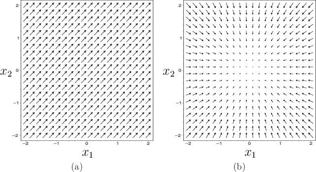
A vector field looks like a ``needle diagram'' over ${\mathbb{R}}^n$, as depicted in Figure 8.5. The idea is to specify a direction at each point $p \in {\mathbb{R}}^n$. When used to represent a feedback plan, it indicates the direction that the robot needs to move if it finds itself at $p$.

For every $p \in {\mathbb{R}}^n$, associate an $n$-dimensional vector space called the tangent space at $p$, which is denoted as $T_p({\mathbb{R}}^n)$. Why not just call it a vector space at $p$? The use of the word ``tangent'' here might seem odd; it is motivated by the generalization to manifolds, for which the tangent spaces will be ``tangent'' to points on the manifold.

A vector field^8.4 ${\vec V}$ on ${\mathbb{R}}^n$ is a function that assigns a vector $v \in T_p({\mathbb{R}}^n)$ to every $p \in {\mathbb{R}}^n$. What is the range of this function? The vector ${\vec V}(p)$ at each $p \in {\mathbb{R}}^n$ actually belongs to a different tangent space. The range of the function is therefore the union

$$T({\mathbb{R}}^n) = \bigcup_{p \in {\mathbb{R}}^n} T_p({\mathbb{R}}^n) ,$$ (8.9)

which is called the tangent bundle on ${\mathbb{R}}^n$. Even though the way we describe vectors from $T_p({\mathbb{R}}^n)$ may appear the same for any $p \in {\mathbb{R}}^n$, each tangent space is assumed to produce distinct vectors. To maintain distinctness, a point in the tangent bundle can be expressed with $2n$ coordinates, by specifying $p$ and $v$ together. This will become important for defining phase space concepts in Part IV. In the present setting, it is sufficient to think of the range of ${\vec V}$ as ${\mathbb{R}}^n$ because $T_p({\mathbb{R}}^n) = {\mathbb{R}}^n$ for every $p \in {\mathbb{R}}^n$.

A vector field can therefore be expressed using $n$ real-valued functions on ${\mathbb{R}}^n$. Let $f_i(x_1,\ldots,x_n)$ for $i$ from $1$ to $n$ denote such functions. Using these, a vector field is specified as

$$f(x) = [f_1(x_1,\ldots,x_n) \;\; f_2(x_1,\ldots,x_n) \;\; \cdots \;\; f_n(x_1,\ldots,x_n)] .$$ (8.10)

In this case, it appears that a vector field is a function $f$ from ${\mathbb{R}}^n$ into ${\mathbb{R}}^n$. Therefore, standard function notation will be used from this point onward to denote a vector field.

Now consider some examples of vector fields over ${\mathbb{R}}^2$. Let a point in ${\mathbb{R}}^2$ be represented as $p = (x,y)$. In standard vector calculus, a vector field is often specified as $[f_1(x,y) \;\;\; f_2(x,y)]$, in which $f_1$ and $f_2$ are functions on ${\mathbb{R}}^2$

Figure: (a) A constant vector field, $f(x,y) = [1\;\;1]$. (b) A vector field, $f(x,y) = [-x\;\;-y]$ in which all vectors point to the origin.

Example 8..6 (Constant Vector Field)   Figure 8.5a shows a constant vector field, which assigns the vector $[1 \;\; 2]$ to every $(x,y) \in {\mathbb{R}}^2$. $\blacksquare$

Example 8..7 (Inward Flow)   Figure 8.5b depicts a vector field that assigns $[-x \;\;\; -y]$ to every $(x,y) \in {\mathbb{R}}^2$. This causes all vectors to point to the origin. $\blacksquare$

Figure: A swirling vector field, $f(x,y) = [(y-x)\;\;(-x-y)]$.

Example 8..8 (Swirl)   The vector field in Figure 8.6 assigns $[(y-x) \;\;\; (-x-y)]$ to every $(x,y) \in {\mathbb{R}}^2$. $\blacksquare$

Due to obstacles that arise in planning problems, it will be convenient to sometimes restrict the domain of a vector field to an open subset of ${\mathbb{R}}^n$. Thus, for any open subset $O \subset {\mathbb{R}}^n$, a vector field $f : O \rightarrow {\mathbb{R}}^n$ can be defined.