3.1.2 Semi-Algebraic Models

In both the polygonal and polyhedral models, $f$ was a linear function. In the case of a semi-algebraic model for a 2D world, $f$ can be any polynomial with real-valued coefficients and variables $x$ and $y$. For a 3D world, $f$ is a polynomial with variables $x$, $y$, and $z$. The class of semi-algebraic models includes both polygonal and polyhedral models, which use first-degree polynomials. A point set determined by a single polynomial primitive is called an algebraic set; a point set that can be obtained by a finite number of unions and intersections of algebraic sets is called a semi-algebraic set.

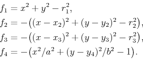
Consider the case of a 2D world. A solid representation can be defined using algebraic primitives of the form

$$H = \{ (x,y) \in {\cal W}\;\vert\; f(x,y) \leq 0 \} .$$ (3.10)

As an example, let $f = x^2 + y^2 - 4$. In this case, $H$ represents a disc of radius $2$ that is centered at the origin. This corresponds to the set of points $(x,y)$ for which $f(x,y) \leq 0$, as depicted in Figure 3.4a.

Figure 3.4: (a) Once again, $f$ is used to partition ${\mathbb{R}}^2$ into two regions. In this case, the algebraic primitive represents a disc-shaped region. (b) The shaded ``face'' can be exactly modeled using only four algebraic primitives.

Example 3..1 (Gingerbread Face)   Consider constructing a model of the shaded region shown in Figure 3.4b. Let the center of the outer circle have radius $r_1$ and be centered at the origin. Suppose that the ``eyes'' have radius $r_2$ and $r_3$ and are centered at $(x_2,y_2)$ and $(x_3,y_3)$, respectively. Let the ``mouth'' be an ellipse with major axis $a$ and minor axis $b$ and is centered at $(0,y_4)$. The functions are defined as

$$\begin{split}f_1 & = x^2 + y^2 - r_1^2, f_2 & = -\big( (x ... ...f_4 & = -\big( x^2/a^2 + (y - y_4)^2/b^2 - 1 \big). \end{split}$$ (3.11)

For $f_2$, $f_3$, and $f_4$, the familiar circle and ellipse equations were multiplied by $-1$ to yield algebraic primitives for all points outside of the circle or ellipse. The shaded region ${\cal O}$ is represented as

$${\cal O}= H_1 \cap H_2 \cap H_3 \cap H_4 .$$ (3.12)

$\blacksquare$

In the case of semi-algebraic models, the intersection of primitives does not necessarily result in a convex subset of ${\cal W}$. In general, however, it might be necessary to form ${\cal O}$ by taking unions and intersections of algebraic primitives.

A logical predicate, $\phi (x,y)$, can once again be formed, and collision checking is still performed in time that is linear in the number of primitives. Note that it is still very efficient to evaluate every primitive; $f$ is just a polynomial that is evaluated on the point $(x,y,z)$.

The semi-algebraic formulation generalizes easily to the case of a 3D world. This results in algebraic primitives of the form

$$H = \{ (x,y,z) \in {\cal W}\;\vert\; f(x,y,z) \leq 0 \} ,$$ (3.13)

which can be used to define a solid representation of a 3D obstacle ${\cal O}$ and a logical predicate $\phi$.

Equations (3.10) and (3.13) are sufficient to express any model of interest. One may define many other primitives based on different relations, such as $f(x,y,z) \geq 0$, $f(x,y,z) = 0$, $f(x,y,z) < 0$, $f(x,y,z) = 0$, and $f(x,y,z) \not = 0$; however, most of them do not enhance the set of models that can be expressed. They might, however, be more convenient in certain contexts. To see that some primitives do not allow new models to be expressed, consider the primitive

$$H = \{ (x,y,z) \in {\cal W}\;\vert\; f(x,y,z) \geq 0 \} .$$ (3.14)

The right part may be alternatively represented as $-f(x,y,z) \leq 0$, and $-f$ may be considered as a new polynomial function of $x$, $y$, and $z$. For an example that involves the $=$ relation, consider the primitive

$$H = \{ (x,y,z) \in {\cal W}\;\vert\; f(x,y,z) = 0 \} .$$ (3.15)

It can instead be constructed as $H = H_1 \cap H_2$, in which

$$H_1 = \{ (x,y,z) \in {\cal W}\;\vert\; f(x,y,z) \leq 0 \}$$ (3.16)

and

$$H_2 = \{ (x,y,z) \in {\cal W}\;\vert\; -f(x,y,z) \leq 0 \} .$$ (3.17)

The relation $<$ does add some expressive power if it is used to construct primitives.^3.2 It is needed to construct models that do not include the outer boundary (for example, the set of all points inside of a sphere, which does not include points on the sphere). These are generally called open sets and are defined Chapter 4.