Next: 12.2.3 Probabilistic Methods for Up: 12.2 Localization Previous: Other information models
Now consider localization for the case in which ![]() is a continuous
region in
is a continuous
region in
![]() . Assume that
. Assume that ![]() is bounded by a simple polygon (a
closed polygonal chain; there are no interior holes). A map of
is bounded by a simple polygon (a
closed polygonal chain; there are no interior holes). A map of ![]() in
in
![]() is given to the robot. The robot velocity
is given to the robot. The robot velocity ![]() is
directly commanded by the action
is
directly commanded by the action ![]() , yielding a motion model
, yielding a motion model
![]() , for which
, for which ![]() is a unit ball centered at the origin. This
enables a plan to be specified as a continuous path in
is a unit ball centered at the origin. This
enables a plan to be specified as a continuous path in ![]() , as was
done throughout Part II. Therefore, instead of specifying
velocities using
, as was
done throughout Part II. Therefore, instead of specifying
velocities using ![]() , a path is directly specified, which is simpler.
For models of the form
, a path is directly specified, which is simpler.
For models of the form
![]() and the more general form
and the more general form
![]() , see Section 8.4 and Chapter 13,
respectively.
, see Section 8.4 and Chapter 13,
respectively.
The robot uses two different sensors:
As in Section 12.2.1, localization involves computing
nondeterministic I-states. In the current setting there is no need to
represent the orientation as part of the state space because of the
perfect compass and known orientation of the polygon in
![]() .
Therefore, the nondeterministic I-states are just subsets of
.
Therefore, the nondeterministic I-states are just subsets of ![]() .
Imagine computing the nondeterministic I-state for the example shown
in Figure 11.15, but without any history. This is
.
Imagine computing the nondeterministic I-state for the example shown
in Figure 11.15, but without any history. This is
![]() , which was defined in (11.6). Only the current
sensor reading is given. This requires computing states from which
the distance measurements shown in Figure 11.15b could be
obtained. This means that a translation must be found that perfectly
overlays the edges shown in Figure 11.15b on top of the
polygon edges that are shown in Figure 11.15a. Let
, which was defined in (11.6). Only the current
sensor reading is given. This requires computing states from which
the distance measurements shown in Figure 11.15b could be
obtained. This means that a translation must be found that perfectly
overlays the edges shown in Figure 11.15b on top of the
polygon edges that are shown in Figure 11.15a. Let
![]() denote the boundary of
denote the boundary of ![]() . The distance measurements
from the visibility sensor must correspond exactly to a subset of
. The distance measurements
from the visibility sensor must correspond exactly to a subset of
![]() . For the example, these could only be obtained from one
state, which is shown in Figure 11.15a. Therefore, the
robot does not even have to move to localize itself for this example.
. For the example, these could only be obtained from one
state, which is shown in Figure 11.15a. Therefore, the
robot does not even have to move to localize itself for this example.
 |
 |
 |
As in Section 8.4.3, let the visibility polygon
![]() refer to the set of all points visible from
refer to the set of all points visible from ![]() , which is
shown in Figure 11.15a. To perform the required
computations efficiently, the polygon must be processed to determine
the different ways in which the visibility polygon could appear from
various points in
, which is
shown in Figure 11.15a. To perform the required
computations efficiently, the polygon must be processed to determine
the different ways in which the visibility polygon could appear from
various points in ![]() . This involves carefully determining which
edges of
. This involves carefully determining which
edges of
![]() could appear on
could appear on
![]() . The state
space
. The state
space ![]() can be decomposed into a finite number of cells, and over
each region the invariant is that same set of edges is used to
describe
can be decomposed into a finite number of cells, and over
each region the invariant is that same set of edges is used to
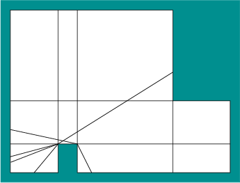
describe ![]() [136,415]. An example is shown
in Figure 12.4. Two different kinds of rays must be
extended to make the decomposition. Figure 12.5 shows
the case in which a pair of vertices is mutually visible and an
outward ray extension is possible. The other case is shown in Figure
12.6, in which rays are extended outward at every
reflex vertex (a vertex whose interior angle is more than
[136,415]. An example is shown
in Figure 12.4. Two different kinds of rays must be
extended to make the decomposition. Figure 12.5 shows
the case in which a pair of vertices is mutually visible and an
outward ray extension is possible. The other case is shown in Figure
12.6, in which rays are extended outward at every
reflex vertex (a vertex whose interior angle is more than ![]() , as
considered in Section 6.2.4). The resulting
decomposition generates
, as
considered in Section 6.2.4). The resulting
decomposition generates ![]() cells in the worse case, in which
cells in the worse case, in which
![]() is the number of edges that form
is the number of edges that form
![]() and
and ![]() is the
number of reflex vertices (note that
is the
number of reflex vertices (note that ![]() ). Once the measurements
are obtained from the sensor, the cell or cells in which the edges or
distance measurements match perfectly need to be computed to determine
). Once the measurements
are obtained from the sensor, the cell or cells in which the edges or
distance measurements match perfectly need to be computed to determine
![]() (the set of points in
(the set of points in ![]() from which the current distance
measurements could be obtained). An algorithm based on the idea of a
visibility skeleton is given in [415], which
performs these computations in time
from which the current distance
measurements could be obtained). An algorithm based on the idea of a
visibility skeleton is given in [415], which
performs these computations in time
![]() and uses
and uses
![]() space, in which
space, in which ![]() is the number of vertices in
is the number of vertices in
![]() ,
, ![]() is the number of vertices in
is the number of vertices in ![]() , and
, and
![]() , the
size of the nondeterministic I-state. This method assumes that the
environment is preprocessed to perform rapid queries during execution;
without preprocessing,
, the
size of the nondeterministic I-state. This method assumes that the
environment is preprocessed to perform rapid queries during execution;
without preprocessing, ![]() can be computed in time
can be computed in time ![]() .
.
 |
What happens if there are multiple states that match the distance data
from the visibility sensor? Since the method in [415]
only computes
![]() , some robot motions must be planned
to further reduce the uncertainty. This provides yet another
interesting illustration of the power of I-spaces. Even though the
state space is continuous, an I-state in this case is used to
disambiguate the state from a finite collection of possibilities.
, some robot motions must be planned
to further reduce the uncertainty. This provides yet another
interesting illustration of the power of I-spaces. Even though the
state space is continuous, an I-state in this case is used to
disambiguate the state from a finite collection of possibilities.
The following example is taken from [298].
The localization problem can be solved in general by using the
visibility cell decomposition, as shown in Figure
12.4. Initially,
![]() is computed
from the initial visibility polygon, which can be efficiently
performed using the visibility skeleton [415]. Suppose
that
is computed
from the initial visibility polygon, which can be efficiently
performed using the visibility skeleton [415]. Suppose
that
![]() contains
contains ![]() states. In this case,
states. In this case, ![]() translated
copies of the map are overlaid so that all of the possible states in
translated
copies of the map are overlaid so that all of the possible states in
![]() coincide. A motion is then executed that reduces the
amount of uncertainty. This could be performed, by example, by
crossing a cell boundary in the overlay that corresponds to one or
more, but not all, of the
coincide. A motion is then executed that reduces the
amount of uncertainty. This could be performed, by example, by
crossing a cell boundary in the overlay that corresponds to one or
more, but not all, of the ![]() copies. This enables some possible
states to be eliminated from the next I-state,
copies. This enables some possible
states to be eliminated from the next I-state,
![]() . The
overlay is used once again to obtain another disambiguating motion,
which results in
. The
overlay is used once again to obtain another disambiguating motion,
which results in
![]() . This process continues until the
state is known. In [298], a motion plan is given that
enables the robot to localize itself by traveling no more than
. This process continues until the
state is known. In [298], a motion plan is given that
enables the robot to localize itself by traveling no more than ![]() times as far as the optimal distance that would need to be traveled to
verify the given state. This particular localization problem might
not seem too difficult after seeing Example 12.3, but it
turns out that the problem of localizing using optimal motions is
NP-hard if any simple polygon is allowed. This was proved in
[298] by showing that every abstract decision tree can be
realized as a localization problem, and the abstract decision tree
problem is already known to be NP-hard.
times as far as the optimal distance that would need to be traveled to
verify the given state. This particular localization problem might
not seem too difficult after seeing Example 12.3, but it
turns out that the problem of localizing using optimal motions is
NP-hard if any simple polygon is allowed. This was proved in
[298] by showing that every abstract decision tree can be
realized as a localization problem, and the abstract decision tree
problem is already known to be NP-hard.
Many interesting variations of the localization problem in continuous
spaces can be constructed by changing the sensing model. For example,
suppose that the robot can only measure distances up to a limit; all
points beyond the limit cannot be seen. This corresponds to many
realistic sensing systems, such as infrared sensors, sonars, and range
scanners on mobile robots. This may substantially enlarge ![]() .
Suppose that the robot can take distance measurements only in a
limited number of directions, as shown in Figure 11.14b.
Another interesting variant can be made by removing the compass. This
introduces the orientation confusion effects observed in Section
12.2.1. One can even consider interesting localization
problems that have little or no sensing [751,752], which
yields I-spaces that are similar to that for the tray tilting example
in Figure 11.28.
.
Suppose that the robot can take distance measurements only in a
limited number of directions, as shown in Figure 11.14b.
Another interesting variant can be made by removing the compass. This
introduces the orientation confusion effects observed in Section
12.2.1. One can even consider interesting localization
problems that have little or no sensing [751,752], which
yields I-spaces that are similar to that for the tray tilting example
in Figure 11.28.
Steven M LaValle 2020-08-14