
Next: 7.7 Optimal Motion Planning Up: 7.6 Coverage Planning Previous: Boustrophedon decomposition
 |
An interesting approximate method was developed by Gabriely and
Rimon; it places a tiling of squares inside of
![]() and computes
the spanning tree of the resulting connectivity graph
[372,373]. Suppose again that
and computes
the spanning tree of the resulting connectivity graph
[372,373]. Suppose again that
![]() is polygonal.
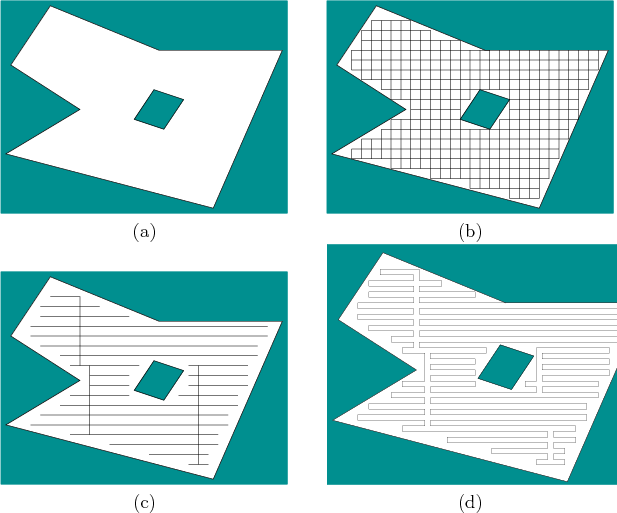
Consider the example shown in Figure 7.37a. The first
step is to tile the interior of
is polygonal.
Consider the example shown in Figure 7.37a. The first
step is to tile the interior of
![]() with squares, as shown in
Figure 7.37b. Each square should be of width
with squares, as shown in
Figure 7.37b. Each square should be of width ![]() ,
for some constant
,
for some constant
![]() . Next, construct a roadmap
. Next, construct a roadmap ![]() by placing a vertex in the center of each square and by defining an
edge that connects the centers of each pair of adjacent cubes. The
next step is to compute a spanning tree of
by placing a vertex in the center of each square and by defining an
edge that connects the centers of each pair of adjacent cubes. The
next step is to compute a spanning tree of ![]() . This is a
connected subgraph that has no cycles and touches every vertex of
. This is a
connected subgraph that has no cycles and touches every vertex of
![]() ; it can be computed in
; it can be computed in ![]() time, if
time, if ![]() has
has ![]() edges
[683]. There are many possible spanning trees, and a
criterion can be defined and optimized to induce preferences. One
possible spanning tree is shown Figure 7.37c.
edges
[683]. There are many possible spanning trees, and a
criterion can be defined and optimized to induce preferences. One
possible spanning tree is shown Figure 7.37c.
 |
Once the spanning tree is made, the robot path is obtained by starting at a point near the spanning tree and following along its perimeter. This path can be precisely specified as shown in Figure 7.38. Double the resolution of the tiling, and form the corresponding roadmap. Part of the roadmap corresponds to the spanning tree, but also included is a loop path that surrounds the spanning tree. This path visits the centers of the new squares. The resulting path for the example of Figure 7.37a is shown in Figure 7.37d. In general, the method yields an optimal route, once the approximation is given. A bound on the uncovered area due to approximation is given in [372]. Versions of the method that do not require an initial map are also given in [372,373]; this involves reasoning about information spaces, which are covered in Chapter 11.
Steven M LaValle 2020-08-14