Next: 7.3.2 Manipulation Planning Up: 7.3 Mixing Discrete and Previous: 7.3 Mixing Discrete and
 |
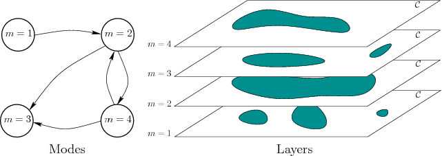
As illustrated in Figure 7.11, a hybrid system involves interaction between discrete and continuous spaces. The formal model will first be given, followed by some explanation. This formulation can be considered as a combination of the components from discrete feasible planning, Formulation 2.1, and basic motion planning, Formulation 4.1.
| (7.13) |
The obstacle region and robot may or may not be mode-dependent, depending on the problem. Examples of each will be given shortly. Changes in the mode depend on the action taken by the robot. From most states, it is usually assumed that a ``do nothing'' action exists, which leaves the mode unchanged. From certain states, the robot may select an action that changes the mode as desired. An interesting degenerate case exists in which there is only a single action available. This means that the robot has no control over the mode from that state. If the robot arrives in such a state, a mode change could unavoidably occur.
The solution requirement is somewhat more complicated because both a
path and an action trajectory need to be specified. It is insufficient
to specify a path because it is important to know what action was
applied to induce the correct mode transitions. Therefore, ![]() indicates when these occur. Note that
indicates when these occur. Note that ![]() and
and ![]() are closely
coupled; one cannot simply associate any
are closely
coupled; one cannot simply associate any ![]() with a path
with a path ![]() ;
it must correspond to the actions required to generate
;
it must correspond to the actions required to generate ![]() .
.
 |
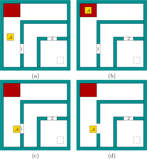
The set, ![]() , of modes needs to encode which key, if any, the robot
holds, and it must also encode the status of the doors. The robot may
have: 1) the key to Door 1; 2) the key to Door 2; or 3) no keys. The
doors may have the status: 1) both open; 2) Door 1 open, Door 2
closed; 3) Door 1 closed, Door 2 open; or 4) both closed. Considering
keys and doors in combination yields
, of modes needs to encode which key, if any, the robot
holds, and it must also encode the status of the doors. The robot may
have: 1) the key to Door 1; 2) the key to Door 2; or 3) no keys. The
doors may have the status: 1) both open; 2) Door 1 open, Door 2
closed; 3) Door 1 closed, Door 2 open; or 4) both closed. Considering
keys and doors in combination yields ![]() possible modes.
possible modes.
If the robot is at a portiernia configuration as shown in Figure
7.12b, then its available actions correspond to
different ways to pick up and drop off keys. For example, if the
robot is holding the key to Door 1, it can drop it off and pick up the
key to Door 2. This changes the mode, but the door status and robot
configuration must remain unchanged when ![]() is applied. The other
locations in which the robot may change the mode are when it comes in
contact with Door 1 or Door 2. The mode changes only if the robot is
holding the proper key. In all other configurations, the robot only
has a single action (i.e., no choice), which keeps the mode fixed.
is applied. The other
locations in which the robot may change the mode are when it comes in
contact with Door 1 or Door 2. The mode changes only if the robot is
holding the proper key. In all other configurations, the robot only
has a single action (i.e., no choice), which keeps the mode fixed.
The task is to reach the configuration shown in the lower right with
dashed lines. The problem is solved by: 1) picking up the key for
Door 1 at the portiernia; 2) opening Door 1; 3) swapping the key at the
portiernia to obtain the key for Door 2; or 4) entering the innermost room
to reach the goal configuration. As a final condition, we might want
to require that the robot returns the key to the portiernia.
![]()
 |
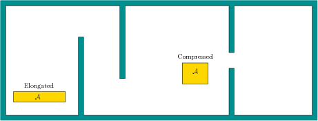
Example 7.2 allows the robot to change the obstacles
in ![]() . The next example involves a robot that can change its shape.
This is an illustrative example of a reconfigurable robot. The
study of such robots has become a popular topic of research
[209,385,552,990]; the reconfiguration
possibilities in that research area are much more complicated than the
simple example considered here.
. The next example involves a robot that can change its shape.
This is an illustrative example of a reconfigurable robot. The
study of such robots has become a popular topic of research
[209,385,552,990]; the reconfiguration
possibilities in that research area are much more complicated than the
simple example considered here.
The examples presented so far barely scratch the surface on the
possible hybrid motion planning problems that can be defined. Many
such problems can arise, for example, in the context making automated
video game characters or digital actors. To solve these problems,
standard motion planning algorithms can be adapted if they are given
information about how to change the modes. Locations in ![]() from
which the mode can be changed may be expressed as subgoals. Much of
the planning effort should then be focused on attempting to change
modes, in addition to trying to directly reach the goal. Applying
sampling-based methods requires the definition of a metric on
from
which the mode can be changed may be expressed as subgoals. Much of
the planning effort should then be focused on attempting to change
modes, in addition to trying to directly reach the goal. Applying
sampling-based methods requires the definition of a metric on ![]() that
accounts for both changes in the mode and the configuration. A wide
variety of hybrid problems can be formulated, ranging from those that
are impossible to solve in practice to those that are straightforward
extensions of standard motion planning. In general, the hybrid motion
planning model is useful for formulating a hierarchical approach, as
described in Section 1.4. One particularly interesting
class of problems that fit this model, for which successful algorithms
have been developed, will be covered next.
that
accounts for both changes in the mode and the configuration. A wide
variety of hybrid problems can be formulated, ranging from those that
are impossible to solve in practice to those that are straightforward
extensions of standard motion planning. In general, the hybrid motion
planning model is useful for formulating a hierarchical approach, as
described in Section 1.4. One particularly interesting
class of problems that fit this model, for which successful algorithms
have been developed, will be covered next.
Steven M LaValle 2020-08-14