7.1.3 The Velocity-Tuning Method

An alternative to defining the problem in ${\cal C}\times T$ is to decouple it into a path planning part and a motion timing part [506]. Algorithms based on this method are not complete, but velocity tuning is an important idea that can be applied elsewhere. Suppose there are both stationary obstacles and moving obstacles. For the stationary obstacles, suppose that some path ${\tau}: [0,1] \rightarrow {\cal C}_{free}$ has been computed using any of the techniques described in Chapters 5 and 6.

The timing part is then handled in a second phase. Design a timing function (or time scaling), ${\sigma}: T \rightarrow [0,1]$, that indicates for time, $t$, the location of the robot along the path, $\tau$. This is achieved by defining the composition ${\phi} = {\tau}\circ {\sigma}$, which maps from $T$ to ${\cal C}_{free}$ via $[0,1]$. Thus, ${\phi}: T \rightarrow {\cal C}_{free}$. The configuration at time $t \in T$ is expressed as ${\phi}(t) = {\tau}({\sigma}(t))$.

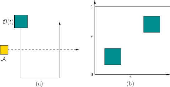
A 2D state space can be defined as shown in Figure 7.4. The purpose is to convert the design of ${\sigma}$ (and consequently ${\phi}$) into a familiar planning problem. The robot must move along its path from $\tau(0)$ to $\tau(1)$ while an obstacle, ${\cal O}(t)$, moves along its path over the time interval $T$. Let $S = [0,1]$ denote the domain of $\tau$. A state space, $X = T \times S$, is shown in Figure 7.4b, in which each point $(t,s)$ indicates the time $t \in T$ and the position along the path, $s \in [0,1]$. The obstacle region in $X$ is defined as

$${X_{obs}}= \{ (t,s) \in X \;\vert\; {\cal A}(\tau(s)) \cap {\cal O}(t) \not = \emptyset \} .$$ (7.5)

Once again, ${X_{free}}$ is defined as ${X_{free}}= X \setminus {X_{obs}}$. The task is to find a continuous path ${g}: [0,1] \rightarrow {X_{free}}$. If ${g}$ is time-monotonic, then a position $s \in S$ is assigned for every time, $t \in T$. These assignments can be nicely organized into the timing function, ${\sigma}: T \rightarrow S$, from which ${\phi}$ is obtained by ${\phi} = {\tau}\circ {\sigma}$ to determine where the robot will be at each time. Being time-monotonic in this context means that the path must always progress from left to right in Figure 7.4b. It can, however, be nonmonotonic in the positive $s$ direction. This corresponds to moving back and forth along $\tau$, causing some configurations to be revisited.

Figure 7.4: An illustration of path tuning. (a) If the robot follows its computed path, it may collide with the moving obstacle. (b) The resulting state space.

Any of the methods described in Formulation 7.1 can be applied here. The dimension of $X$ in this case is always $2$. Note that ${X_{obs}}$ is polygonal if ${\cal A}$ and ${\cal O}$ are both polygonal regions and their paths are piecewise-linear. In this case, the vertical decomposition method of Section 6.2.2 can be applied by sweeping along the time axis to yield a complete algorithm (it is complete after having committed to $\tau$, but it is not complete for Formulation 7.1). The result is shown in Figure 7.5. The cells are connected only if it is possible to reach one from the other by traveling in the forward time direction. As an example of a sampling-based approach that may be preferable when ${X_{obs}}$ is not polygonal, place a grid over $X$ and apply one of the classical search algorithms described in Section 5.4.2. Once again, only path segments in $X$ that move forward in time are allowed.

Figure 7.5: Vertical cell decomposition can solve the path tuning problem. Note that this example is not in general position because vertical edges exist. The goal is to reach the horizontal line at the top, which can be accomplished from any adjacent $2$-cell. For this example, it may even be accomplished from the first $2$-cell if the robot is able to move quickly enough.