9.5.1.3 Constructing a utility function

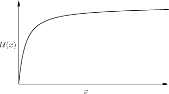
If the preferences have been determined in a way consistent with the axioms, then it can be shown that a utility function always exists. This means that there exists a function ${\cal U}: X \rightarrow {\mathbb{R}}$ such that, for all $z_1, z_2 \in Z$,

$$z_1 \prec z_2 E_{z_1}[{\cal U}] < E_{z_2}[{\cal U}] ,$$ (9.87)

in which $E_{z_i}$ denotes the expected value of ${\cal U}$, which is being treated as a random variable under the probability distribution $z_i$. The existence of ${\cal U}$ implies that it is safe to determine the best action by maximizing the expected utility.

A reward function can be defined using a utility function, ${\cal U}$, as $R(u,\theta) = {\cal U}(f(u,\theta))$. The utility function can be converted to a cost function as $L(u,\theta) = -R(u,\theta) = -{\cal U}(f(u,\theta))$. Minimizing the expected cost, as was recommended under Formulations 9.3 and 9.4 with probabilistic uncertainty, now seems justified under the assumption that ${\cal U}$ was constructed correctly to preserve preferences.

Unfortunately, establishing the existence of a utility function does not produce a systematic way to construct it. In most circumstances, one is forced to design ${\cal U}$ by a trial-and-error process that involves repeatedly checking the preferences. In the vast majority of applications, people create utility and cost functions without regard to the implications discussed in this section. Thus, undesirable conclusions may be reached in practice. Therefore, it is important not to be too confident about the quality of an optimal decision rule.

Note that if worst-case analysis had been used, then most of the problems discussed here could have been avoided. Worst-case analysis, however, has its weaknesses, which will be discussed in Section 9.5.3.

Example 9..25 (The Utility of Money)   We conclude the section by depicting a utility function that is often applied to money. Suppose that the state space $X = {\mathbb{R}}$, which corresponds to the amount of U.S. dollars earned. The utility of money applied by most people indicates that the value of new increments of money decreases as the total accumulated wealth increases. The utility function may even be bounded. Imagine there is some maximum dollar amount, such as $$10^{100}$, after which additional money has no value. A typical utility curve is shown in Figure 9.6 [89].

Figure 9.6: The utility of new amounts of money decreases as the total accumulation of wealth increases. The utility function may even bounded.

$\blacksquare$