What if there are loops?

Figure 3.26: There are ten links and ten revolute joints arranged in a loop. This is an example of a closed kinematic chain.

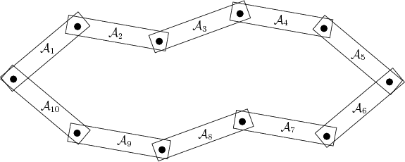
The most general case includes links that are connected in loops, as shown in Figure 3.26. These are generally referred to as closed kinematic chains. This arises in many applications. For example, with humanoid robotics or digital actors, a loop is formed when both feet touch the ground. As another example, suppose that two robot manipulators, such as the Puma 560 from Example 3.4, cooperate together to carry an object. If each robot grasps the same object with its hand, then a loop will be formed. A complicated example of this was shown in Figure 1.5, in which mobile robots moved a piano. Outside of robotics, a large fraction of organic molecules have flexible loops. Exploring the space of their conformations requires careful consideration of the difficulties imposed by these loops.

Figure 3.27: Loops may be opened to enable tree-based transformations to be applied; however, a closure constraint must still be satisfied.

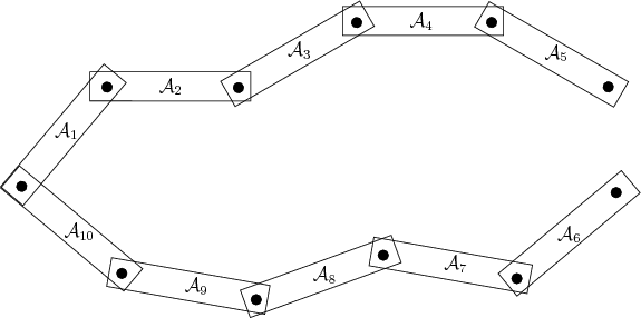
The main difficulty of working with closed kinematic chains is that it is hard to determine which parameter values are within an acceptable range to ensure closure. If these values are given, then the transformations are handled in the same way as the case of trees. For example, the links in Figure 3.26 may be transformed by breaking the loop into two different chains. Suppose we forget that the joint between ${\cal A}_5$ and ${\cal A}_6$ exists, as shown in Figure 3.27. Consider two different kinematic chains that start at the joint on the extreme left. There is an upper chain from ${\cal A}_1$ to ${\cal A}_5$ and a lower chain from ${\cal A}_{10}$ to ${\cal A}_6$. The transformations for any of these bodies can be obtained directly from the techniques of Section 3.3.1. Thus, it is easy to transform the bodies, but how do we choose parameter values that ensure ${\cal A}_5$ and ${\cal A}_6$ are connected at their common joint? Using the upper chain, the position of this joint may be expressed as

$$T_1(\theta_1) T_2(\theta_2) T_3(\theta_3) T_4(\theta_4) T_5(\theta_5) \begin{pmatrix}a_5 0 1 \end{pmatrix} ,$$ (3.79)

in which $(a_5,0) \in {\cal A}_5$ is the location of the joint of ${\cal A}_5$ that is supposed to connect to ${\cal A}_6$. The position of this joint may also be expressed using the lower chain as

$$T_{10}(\theta_{10}) T_9(\theta_9) T_8(\theta_8) T_7(\theta_7) T_6(\theta_6) \begin{pmatrix}a_6 0 1 \end{pmatrix} ,$$ (3.80)

with $(a_6,0)$ representing the position of the joint in the body frame of ${\cal A}_6$. If the loop does not have to be maintained, then any values for $\theta_1$, $\ldots$, $\theta_{10}$ may be selected, resulting in ten degrees of freedom. However, if a loop must maintained, then (3.79) and (3.80) must be equal,

$$T_1(\theta_1) T_2(\theta_2) T_3(\theta_3) T_4(\theta_4) T_5(\thet... ..._8) T_7(\theta_7) T_6(\theta_6) \begin{pmatrix}a_6 0 1 \end{pmatrix} ,$$ (3.81)

which is quite a mess of nonlinear, trigonometric equations that must be solved. The set of solutions to (3.81) could be very complicated. For the example, the true degrees of freedom is eight because two were removed by making the joint common. Since the common joint allows the links to rotate, exactly two degrees of freedom are lost. If ${\cal A}_5$ and ${\cal A}_6$ had to be rigidly attached, then the total degrees of freedom would be only seven. For most problems that involve loops, it will not be possible to obtain a nice parameterization of the set of solutions. This a form of the well-known inverse kinematics problem [252,693,775,994].

In general, a complicated arrangement of links can be imagined in which there are many loops. Each time a joint along a loop is ``ignored,'' as in the procedure just described, then one less loop exists. This process can be repeated iteratively until there are no more loops in the graph. The resulting arrangement of links will be a tree for which the previous techniques of this section may be applied. However, for each joint that was ``ignored'' an equation similar to (3.81) must be introduced. All of these equations must be satisfied simultaneously to respect the original loop constraints. Suppose that a set of value parameters is already given. This could happen, for example, using motion capture technology to measure the position and orientation of every part of a human body in contact with the ground. From this the solution parameters could be computed, and all of the transformations are easy to represent. However, as soon as the model moves, it is difficult to ensure that the new transformations respect the closure constraints. The foot of the digital actor may push through the floor, for example. Further information on this problem appears in Section 4.4.