Numerical wave propagation

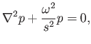
The Helmholtz wave equation expresses constraints at every point in ${\mathbb{R}}^3$ in terms of partial derivatives of the pressure function. Its frequency-dependent form is

$$\nabla^2 p + \frac{\omega^2}{s^2} p = 0 ,$$ (11.8)

in which $p$ is the sound pressure, $\nabla^2$ is the Laplacian operator from calculus, and $\omega$ is related to the frequency $f$ as $\omega = 2 \pi f$.

Figure 11.14: Computed results for sound propagation by numerically solving the Helmholtz wave equation (taken from [211]): (a) The pressure magnitude before obstacle interaction is considered. (b) The pressure after taking into account scattering. (c) The scattering component, which is the pressure from (b) minus the pressure from (a).

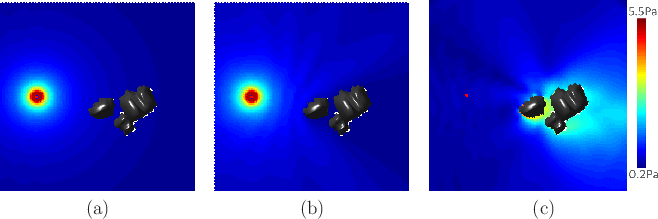Closed-form solutions to (11.8) do not exist, except in trivial cases. Therefore, numerical computations are performed by iteratively updating values over the space; a brief survey of methods in the context of auditory rendering appears in [211]. The wave equation is defined over the obstacle-free portion of the virtual world. The edge of this space becomes complicated, leading to boundary conditions. One or more parts of the boundary correspond to sound sources, which can be considered as vibrating objects or obstacles that force energy into the world. At these locations, the 0 in (11.8) is replaced by a forcing function. At the other boundaries, the wave may undergo some combination of absorption, reflection, scattering, and diffraction. These are extremely difficult to model; see [268] for details. In some rendering applications, these boundary interactions may simplified and handled with simple Dirichlet boundary conditions and Neumann boundary conditions [369]. If the virtual world is unbounded, then an additional Sommerfield radiation condition is needed. For detailed models and equations for sound propagation in a variety of settings, see [268]. An example of a numerically computed sound field is shown in Figure 11.14.