Reverse-time system simulation

Some planning algorithms require integration in the reverse-time direction. For some given $x(0)$ and action trajectory that runs from $-\Delta t$ to 0, the backward system simulator computes a state trajectory, ${\tilde{x}}: [-t,0] \rightarrow X$, which when integrated from $-\Delta t$ to 0 under the application of ${\tilde{u}}_t$ yields $x(0)$. This may seem like an inverse control problem [856] or a BVP as shown in Figure 14.10; however, it is much simpler. Determining the action trajectory for given initial and goal states is more complicated; however, in reverse-time integration, the action trajectory and final state are given, and the initial state does not need to be fixed.

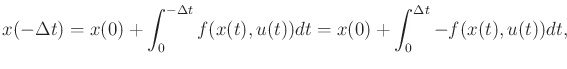
The reverse-time version of (14.14) is

$$x(-\Delta t) = x(0) + \int_{0}^{-\Delta t} f(x(t),u(t)) dt = x(0) + \int_{0}^{\Delta t} -f(x(t),u(t)) dt ,$$ (14.20)

which relies on the fact that ${\dot x}= f(x,u)$ is time-invariant. Thus, reverse-time integration is obtained by simply negating the state transition equation. The Euler and Runge-Kutta methods can then be applied in the usual way to $-f(x(t),u(t))$.