12.2.1 Discrete Localization

Many interesting lessons about realistic localization problems can be learned by first studying a discrete version of localization. Problems that may or may not be solvable can be embedded in more complicated problems, which may even involve continuous state spaces. The discrete case is often easier to understand, which motivates its presentation here. To simplify the presentation, only the nondeterministic I-space ${\cal I}_{ndet}$ will be considered; see Section 12.2.3 for the probabilistic case.

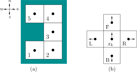
Suppose that a robot moves on a 2D grid, which was introduced in Example 2.1. It has a map of the grid but does not know its initial location or orientation within the grid. An example is shown in Figure 12.2a.

Figure 12.2: (a) This map is given to the robot for localization purposes. (b) The four possible actions each take one step, if possible, and reorient the robot as shown.

To formulate the problem, it is helpful to include in the state both the position of the robot and its orientation. Suppose that the robot may be oriented in one of four directions, which are labeled N, E, W, and S, for ``north,'' ``east,'' ``west,'' and ``south,'' respectively. Although the robot is treated as a point, its orientation is important because it does not have a compass. If it chooses to move in a particular direction, such as straight ahead, it does not necessarily know which direction it will be heading with respect to the four directions.

Thus, a state, $x \in X$, is written as $x = (p,d)$, in which $p$ is a position and $d$ is one of the four directions. A set of states at the same position will be denoted with special superscripts that point in the possible directions. For example, $3^{\psfig{figure=figs/locplus3.eps,width=3mm}}$ indicates the set of states for which $p = 3$ and the direction may be north (N) or east (E), because the superscript points in the north and east directions.

Figure 12.3: (a) If a direction is blocked because of an obstacle, then the orientation changes, but the position remains fixed. In this example, the $R$ action is applied. (b) Another map is given to the robot for localization purposes. In this case, the robot cannot localize itself exactly.

The robot is given four actions,

$$U = \{{\rm F},{\rm B},{\rm R},{\rm L}\},$$ (12.11)

which represent ``forward,'' ``backward,'' ``right motion,'' and ``left motion,'' respectively. These motions occur with respect to the current orientation of the robot, which may be unknown. See Figure 12.2b. For the $F$ action, the robot moves forward one grid element and maintains its orientation. For the $B$ action, the robot changes its orientation by $180$ degrees and then moves forward one grid element. For the R action, the robot turns right by $90$ degrees and then moves forward one grid element. The L action behaves similarly. If it is not possible to move because of an obstacle, it is assumed that the robot changes its orientation (in the case of B, R, or L) but does not change its position. This is depicted in Figure 12.3a.

The robot has one simple sensor that can only detect whether it was able to move in the direction that was attempted. The sensor space is $Y = \{0,1\}$, and the sensor mapping is $h : X \times X \rightarrow Y$. This yields $y = h(x_{k-1},x_k) = 1$ if $x_{k-1}$ and $x_k$ place the robot at different positions, and $h(x_{k-1},x_k) = 0$ otherwise. Thus, the sensor indicates whether the robot has moved after the application of an action.

Nondeterministic uncertainty will be used, and the initial I-state ${\eta_0}$ is always assumed to be $X$ (this can easily be extended to allow starting with any nonempty subset of $X$). A history I-state at stake $k$ in its general form appears as

$${\eta}_0 = (X,{\tilde{u}}_{k-1},y_2,\ldots,y_k) .$$ (12.12)

One special adjustment was made in comparison to (11.14). There is no observation $y_1$ because the sensor mapping requires a previous state to report a value. Thus, the observation history starts with $y_2$. An example history I-state for stage $k=5$ is

$${\eta}_5 = (X, {\rm R}, {\rm R}, {\rm F}, {\rm L}, 1,0,1,1) ,$$ (12.13)

in which ${\eta_0}= X$, ${\tilde{u}}_4 = ({\rm R},{\rm R},{\rm F},{\rm L})$, and $(y_2,y_3,y_4,y_5) = (1,0,1,1)$.

The passive localization problem starts with a given map, such as the one shown in Figure 12.2a, and a history I-state, ${\eta}_k$, and computes the nondeterministic I-state $X_k({\eta}_k) \subseteq X$. The active localization problem is to compute some $k$ and sequence of actions, $(u_1,\ldots,u_{k-1})$, such that the nondeterministic I-state is as small as possible. In the best case, $X_k({\eta}_k)$ might become a singleton set, which means that the robot knows its position and orientation on the map. However, due to symmetries, which will be presented shortly in an example, it might not be possible.