Next: Two screws Up: 3.3 Transforming Kinematic Chains Previous: Homogeneous transformation matrices for
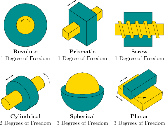
As for a single rigid body, the 3D case is significantly more complicated than the 2D case due to 3D rotations. Also, several more types of joints are possible, as shown in Figure 3.12. Nevertheless, the main ideas from the transformations of 2D kinematic chains extend to the 3D case. The following steps from Section 3.3.1 will be recycled here:
Consider a kinematic chain of ![]() links in
links in
![]() , in which each
, in which each
![]() for
for
![]() is attached to
is attached to
![]() by a revolute
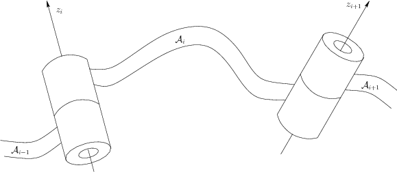
joint. Each link can be a complicated, rigid body as shown in Figure
3.13. For the 2D problem, the coordinate frames were based
on the points of attachment. For the 3D problem, it is convenient to
use the axis of rotation of each revolute joint (this is
equivalent to the point of attachment for the 2D case). The axes of
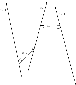
rotation will generally be skew lines in
by a revolute
joint. Each link can be a complicated, rigid body as shown in Figure
3.13. For the 2D problem, the coordinate frames were based
on the points of attachment. For the 3D problem, it is convenient to
use the axis of rotation of each revolute joint (this is
equivalent to the point of attachment for the 2D case). The axes of
rotation will generally be skew lines in
![]() , as shown in Figure
3.14. Let the
, as shown in Figure
3.14. Let the ![]() -axis be the axis of rotation for
the revolute joint that holds
-axis be the axis of rotation for
the revolute joint that holds
![]() to
to
![]() . Between
each pair of axes in succession, let the
. Between
each pair of axes in succession, let the ![]() -axis join the closest
pair of points between the
-axis join the closest
pair of points between the ![]() - and
- and ![]() -axes, with the origin
on the
-axes, with the origin
on the ![]() -axis and the direction pointing towards the nearest point
of the
-axis and the direction pointing towards the nearest point
of the ![]() -axis. This axis is uniquely defined if the
-axis. This axis is uniquely defined if the ![]() -
and
-
and ![]() -axes are not parallel. The recommended body frame for
each
-axes are not parallel. The recommended body frame for
each
![]() will be given with respect to the
will be given with respect to the ![]() - and
- and ![]() -axes,
which are shown in Figure 3.14. Assuming a
right-handed coordinate system, the
-axes,
which are shown in Figure 3.14. Assuming a
right-handed coordinate system, the ![]() -axis points away from us in
Figure 3.14. In the transformations that will appear
shortly, the coordinate frame given by
-axis points away from us in
Figure 3.14. In the transformations that will appear
shortly, the coordinate frame given by ![]() ,
, ![]() , and
, and ![]() will
be most convenient for defining the model for
will
be most convenient for defining the model for
![]() . It might not
always appear convenient because the origin of the frame may even lie
outside of
. It might not
always appear convenient because the origin of the frame may even lie
outside of
![]() , but the resulting transformation matrices will be
easy to understand.
, but the resulting transformation matrices will be
easy to understand.
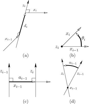 |
In Section 3.3.1, each ![]() was defined in terms of two
parameters,
was defined in terms of two
parameters, ![]() and
and ![]() . For the 3D case, four
parameters will be defined:
. For the 3D case, four
parameters will be defined: ![]() ,
, ![]() ,
, ![]() , and
, and
![]() . These are referred to as Denavit-Hartenberg (DH)
parameters [434]. The
definition of each parameter is indicated in Figure 3.15.
Figure 3.15a shows the definition of
. These are referred to as Denavit-Hartenberg (DH)
parameters [434]. The
definition of each parameter is indicated in Figure 3.15.
Figure 3.15a shows the definition of ![]() . Note that the
. Note that the
![]() - and
- and ![]() -axes contact the
-axes contact the ![]() -axis at two different
places. Let
-axis at two different
places. Let ![]() denote signed distance between these points of
contact. If the
denote signed distance between these points of
contact. If the ![]() -axis is above the
-axis is above the ![]() -axis along the
-axis along the
![]() -axis, then
-axis, then ![]() is positive; otherwise,
is positive; otherwise, ![]() is negative. The
parameter
is negative. The
parameter ![]() is the angle between the
is the angle between the ![]() - and
- and
![]() -axes, which corresponds to the rotation about the
-axes, which corresponds to the rotation about the ![]() -axis
that moves the
-axis
that moves the ![]() -axis to coincide with the
-axis to coincide with the ![]() -axis. The
parameter
-axis. The
parameter ![]() is the distance between the
is the distance between the ![]() - and
- and ![]() -axes;
recall these are generally skew lines in
-axes;
recall these are generally skew lines in
![]() . The parameter
. The parameter
![]() is the angle between the
is the angle between the ![]() - and
- and ![]() -axes.
-axes.