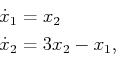
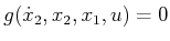
To make the discussion concrete, consider the following differential
equation:
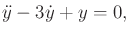 |
(13.29) |
in which  is a scalar variable,
 . This is a
second-order differential equation because of
. This is a
second-order differential equation because of  . A phase
space can be defined as follows. Let
. A phase
space can be defined as follows. Let
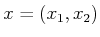 denote a
two-dimensional phase vector, which is defined by assigning
denote a
two-dimensional phase vector, which is defined by assigning
 and
and
 . The terms state space and state vector will be
used interchangeably with phase space and phase vector, respectively,
in contexts in which the phase space is defined. Substituting the
equations into (13.29) yields
. The terms state space and state vector will be
used interchangeably with phase space and phase vector, respectively,
in contexts in which the phase space is defined. Substituting the
equations into (13.29) yields
 |
(13.30) |
So far, this does not seem to have helped. However, can be
expressed as either
 or
or
 . The first choice is
better because it is a lower order derivative. Using
. The first choice is
better because it is a lower order derivative. Using
 , the differential equation becomes
 |
(13.31) |
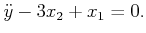
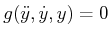
Is this expression equivalent to (13.29)? By itself it is
not. There is one more constraint,
 . In implicit
form,
. In implicit
form,
 . The key to making the phase space approach
work correctly is to relate some of the phase variables by
derivatives.
. The key to making the phase space approach
work correctly is to relate some of the phase variables by
derivatives.
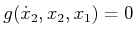
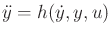
Using the phase space, we just converted the second-order differential
equation (13.29) into two first-order differential
equations,
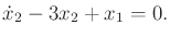
 |
(13.32) |
which are obtained by solving for
 and
. Note that
(13.32) can be expressed as
and
. Note that
(13.32) can be expressed as
 , in which
  is a function that maps from
 into
.
into
.
The same approach can be used for any differential equation in
implicit form,
 . Let ,
,
and
. This results in the implicit equations
. Let ,
,
and
. This results in the implicit equations
 and
and
 . Now suppose that there
is a scalar action
. Now suppose that there
is a scalar action
 represented in the differential
equations. Once again, the same approach applies. In implicit form,
represented in the differential
equations. Once again, the same approach applies. In implicit form,
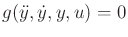 can be expressed as
 .
.
Suppose that a given acceleration constraint is expressed in
parametric form as
 . This often occurs in the
dynamics models of Section 13.3. This can be converted
into a phase transition equation or state transition
equation of the form
. This often occurs in the
dynamics models of Section 13.3. This can be converted
into a phase transition equation or state transition
equation of the form
 , in which
 . The expression is
 |
(13.33) |
For a second-order differential equation, two initial conditions are
usually given. The values of  and
and
 are needed to
determine the exact position
are needed to
determine the exact position  for any
  . Using the
phase space representation, no higher order initial conditions are
needed because any point in phase space indicates both and
. Using the
phase space representation, no higher order initial conditions are
needed because any point in phase space indicates both and
 . Thus, given an initial point in the phase and
  for all
, can be determined.
for all
, can be determined.
Example 13..3 (Double Integrator)
The
double integrator is a simple
yet important example that nicely illustrates the phase space.
Suppose that a second-order differential equation is given as

, in which

and

are chosen from

. In words, this
means that the action directly specifies acceleration.
Integrating
13.5 once yields the velocity

and performing a double integration yields the position
.
If

and

are given, and

is specified for all

, then

and

can be determined for any

.
A two-dimensional phase space
 is defined in which
 |
(13.34) |
The state (or phase) transition equation
is
 |
(13.35) |
To determine the state trajectory, initial values

(position) and

(velocity) must be given in addition
to the action history. If
is constant, then the state trajectory
is quadratic because it is obtained by two integrations of a constant
function.

Steven M LaValle
2020-08-14
