Next: 13.1.2 Kinematics for Wheeled Up: 13.1.1 Implicit vs. Parametric Previous: 13.1.1.2 Parametric constraints
There are trade-offs between the implicit and parametric ways to express differential constraints. The implicit representation is more general; however, the parametric form is more useful because it explicitly gives the possible actions. For this reason, it is often desirable to derive a parametric representation from an implicit one. Under very general conditions, it is theoretically possible. As will be explained shortly, this is a result of the implicit function theorem. Unfortunately, the theoretical existence of such a conversion does not help in actually performing the transformations. In many cases, it may not be practical to determine a parametric representation.
To model a mechanical system, it is simplest to express constraints in
the implicit form and then derive the parametric representation
![]() . So far there has been no appearance of
. So far there has been no appearance of ![]() in the implicit
representation. Since
in the implicit
representation. Since ![]() is interpreted as an action, it needs to be
specified while deriving the parametric representation. To understand
the issues, it is helpful to first assume that all constraints in
implicit form are linear equations in
is interpreted as an action, it needs to be
specified while deriving the parametric representation. To understand
the issues, it is helpful to first assume that all constraints in
implicit form are linear equations in ![]() of the form
of the form
Suppose that ![]() Pfaffian constraints are given for
Pfaffian constraints are given for ![]() and
that they are linearly independent.13.1 Recall the
standard techniques for solving linear equations. If
and
that they are linearly independent.13.1 Recall the
standard techniques for solving linear equations. If ![]() , then a
unique solution exists. If
, then a
unique solution exists. If ![]() , then a continuum of solutions
exists, which forms an
, then a continuum of solutions
exists, which forms an ![]() -dimensional hyperplane. It is
impossible to have
-dimensional hyperplane. It is
impossible to have ![]() because there can be no more than
because there can be no more than ![]() linearly independent equations.
linearly independent equations.
If ![]() , only one velocity vector satisfies the constraints for
each
, only one velocity vector satisfies the constraints for
each
![]() . A vector field can therefore be derived from the
constraints, and the problem is not interesting from a planning
perspective because there is no choice of velocities. If
. A vector field can therefore be derived from the
constraints, and the problem is not interesting from a planning
perspective because there is no choice of velocities. If ![]() ,
then
,
then ![]() components of
components of ![]() can be chosen independently, and then
the remaining
can be chosen independently, and then
the remaining ![]() are computed to satisfy the Pfaffian constraints
(this can be accomplished using linear algebra techniques such as
singular value decomposition [399,961]). The components of
are computed to satisfy the Pfaffian constraints
(this can be accomplished using linear algebra techniques such as
singular value decomposition [399,961]). The components of
![]() that can be chosen independently can be considered as
that can be chosen independently can be considered as ![]() scalar actions. Together these form an
scalar actions. Together these form an ![]() -dimensional action
vector,
-dimensional action
vector,
![]() . Suppose without loss of
generality that the first
. Suppose without loss of
generality that the first ![]() components of
components of ![]() are specified by
are specified by
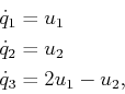
![]() . The configuration transition equation can then be written as
. The configuration transition equation can then be written as
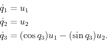
The constraint given in (13.7) does not even depend on
![]() . The same ideas apply for more general Pfaffian constraints, such
as
. The same ideas apply for more general Pfaffian constraints, such
as
The ideas presented so far naturally extend to equality constraints
that are not linear in ![]() . At each
. At each ![]() , an
, an ![]() -dimensional
set of actions,
-dimensional
set of actions, ![]() , is guaranteed to exist if the Jacobian
, is guaranteed to exist if the Jacobian
![]() (recall
(6.28) or see [508]) of the constraint functions
has rank
(recall
(6.28) or see [508]) of the constraint functions
has rank ![]() at
at ![]() . This follows from the implicit function
theorem [508].
. This follows from the implicit function
theorem [508].
Suppose that there are inequality constraints of the form
![]() , in addition to equality constraints. Using the previous
concepts, the actions may once again be assigned directly as
, in addition to equality constraints. Using the previous
concepts, the actions may once again be assigned directly as
![]() for all
for all ![]() such that
such that
![]() . Without inequality
constraints, there are no constraints on
. Without inequality
constraints, there are no constraints on ![]() , which means that
, which means that
![]() . Since
. Since ![]() is interpreted as an input to some physical system,
is interpreted as an input to some physical system,
![]() will often be constrained. In a physical system, for example, the
amount of energy consumed may be proportional to
will often be constrained. In a physical system, for example, the
amount of energy consumed may be proportional to ![]() . After
performing the
. After
performing the
![]() substitutions, the inequality
constraints indicate limits on
substitutions, the inequality
constraints indicate limits on ![]() . These limits are expressed in
terms of
. These limits are expressed in
terms of ![]() and the remaining components of
and the remaining components of ![]() , which are the
variables
, which are the
variables
![]() ,
, ![]() ,
,
![]() . For many problems,
the inequality constraints are simple enough that constraints directly
on
. For many problems,
the inequality constraints are simple enough that constraints directly
on ![]() can be derived. For example, if
can be derived. For example, if ![]() represents scalar
acceleration applied to a car, then it may have a simple bound such as
represents scalar
acceleration applied to a car, then it may have a simple bound such as
![]() .
.
One final complication that sometimes occurs is that the action
variables may already be specified in the equality constraints:
![]() . In this case, imagine once again that
. In this case, imagine once again that ![]() is
fixed. If there are
is
fixed. If there are ![]() independent constraints, then by the implicit
function theorem,
independent constraints, then by the implicit
function theorem, ![]() can be solved to yield
can be solved to yield
![]() (although theoretically possible, it may be difficult in practice).
If the Jacobian
(although theoretically possible, it may be difficult in practice).
If the Jacobian
![]() has rank
has rank ![]() at
at ![]() , then actions can be applied to
yield any velocity on a
, then actions can be applied to
yield any velocity on a ![]() -dimensional hyperplane in
-dimensional hyperplane in
![]() . If
. If
![]() , then there are enough independent action variables to
overcome the constraints. Any velocity in
, then there are enough independent action variables to
overcome the constraints. Any velocity in
![]() can be achieved
through a choice of
can be achieved
through a choice of ![]() . This is true only if there are no inequality
constraints on
. This is true only if there are no inequality
constraints on ![]() .
.
Steven M LaValle 2020-08-14