11.5.2 Simple Projection Examples

This section gives examples of I-spaces for which the sensor mapping is $y = h(x)$ and $h$ is a projection that reveals some of the state variables, while concealing others. The examples all involve continuous time, and the focus is mainly on the nondeterministic I-space ${\cal I}_{ndet}$. It is assumed that there are no actions, which means that $U = \emptyset$. Nature actions, $\Theta(x)$, however, will be allowed. Since there are no robot actions and no nature sensing actions, all of the uncertainty arises from the fact that $h$ is a projection and the nature actions that affect the state transition equation are not known. This is a very important and interesting class of problems in itself. The examples can be further complicated by allowing some control from the action set, $U$; however, the purpose here is to illustrate I-space concepts. Therefore, it will not be necessary.

Figure 11.17: The state space is the set of points traced out by a sine curve in ${\mathbb{R}}^2$.

Example 11..20 (Moving on a Sine Curve)   Suppose that the state space is the set of points that lie on the sine curve in the plane:

$$X = \{ (x_1,x_2) \in {\mathbb{R}}^2 \;\vert\; x_2 = \sin x_1 \} .$$ (11.72)

Let $U = \emptyset$, which results in no action history. The observation space is $Y = [-1,1]$ and the sensor mapping yields $y = h(x) = x_2$, the height of the point on the sine curve, as shown in Figure 11.17.

The nature action space is $\Theta = \{-1,1\}$, in which $-1$ means to move at unit speed in the $-x_1$ direction along the sine curve, and $1$ means to move at unit speed in the $x_1$ direction along the curve. Thus, for some nature action history ${\tilde{\theta}_t}$, a state trajectory ${\tilde{x}_t}$ that moves the point along the curve can be determined by integration.

Figure 11.18: The preimage, $H(y)$, of an observation $y$ is a countably infinite set of points along $X$.

A history I-state takes the form ${\eta}_t = (X_0,{\tilde{y}_t})$, which includes the initial condition $X_0 \subseteq X$ and the observation history ${\tilde{y}_t}$ up to time $t$. The nondeterministic I-states are very interesting for this problem. For each observation $y$, the preimage $H(y)$ is a countably infinite set of points that corresponds to the intersection of $X$ with a horizontal line at height $y$, as shown in Figure 11.18.

The uncertainty for this problem is always characterized by the number of intersection points that might contain the true state. Suppose that $X_0 = X$. In this case, there is no state trajectory that can reduce the amount of uncertainty. As the point moves along $X$, the height is always known because of the sensor, but the $x_1$ coordinate can only be narrowed down to being any of the intersection points.

Figure 11.19: A bifurcation occurs when $y=1$ or $y=-1$ is received. This irreversibly increases the amount of uncertainty in the state.

Suppose instead that $X_0 = \{x_0\}$, in which $x_0$ is some particular point along $X$. If $y$ remains within $(0,1)$ over some any period of time starting at $t=0$, then $x(t)$ is known because the exact segment of the sine curve that contains the state is known. However, if the point reaches an extremum, which results in $y=0$ or $y=1$, then it is not known which way the point will travel. From this point, the sensor cannot disambiguate moving in the $-x_1$ direction from the $x_1$ direction. Therefore, the uncertainty grows, as shown in Figure 11.19. After the observation $y=1$ is obtained, there are two possibilities for the current state, depending on which action was taken by nature when $y=1$; hence, the nondeterministic I-state contains two states. If the motion continues until $y=-1$, then there will be four states in the nondeterministic I-state. Unfortunately, the uncertainty can only grow in this example. There is no way to use the sensor to reduce the size of the nondeterministic I-states. $\blacksquare$

Figure 11.20: (a) Imagine trying to infer the location of a point on a planar graph while observing only a single coordinate. (b) This simple example involves a point moving along a graph that has four edges. When the point is on the rightmost edge, there is no uncertainty; however, uncertainty exists when the point travels along the other edges.

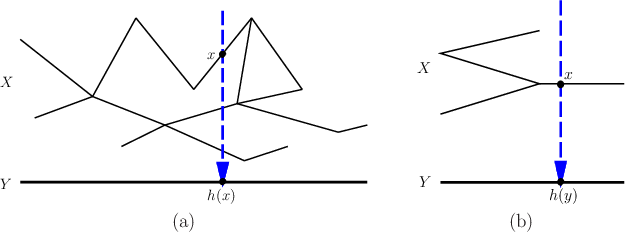
The previous example can be generalized to observing a single coordinate of a point that moves around in a planar topological graph, as shown in Figure 11.20a. Most of the model remains the same as for Example 11.20, except that the state space is now a graph. The set of nature actions, $\Theta(x)$, needs to be extended so that if $x$ is a vertex of the graph, then there is one input for each incident edge. These are the possible directions along which the point could move.

Figure 11.21: Pieces of the nondeterministic I-space ${\cal I}_{ndet}$ are obtained by the different possible sets of edges on which the point may lie.

Example 11..21 (Observing a Point on a Graph)   Consider the graph shown in Figure 11.20b, in which there are four edges.^11.8 When the point moves on the interior of the rightmost edge of the graph, then the state can be inferred from the sensor. The set $H(y)$ contains a single point on the rightmost edge. If the point moves in the interior of one of the other edges, then $H(y)$ contains three points, one for each edge above $y$. This leads to seven possible cases for the nondeterministic I-state, as shown in Figure 11.21. Any subset of these edges may be possible for the nondeterministic I-state, except for the empty set.

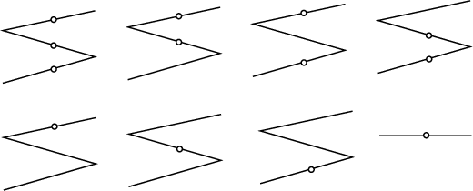
The eight pieces of ${\cal I}_{ndet}$ depicted in Figure 11.21 are connected together in an interesting way. Suppose that the point is on the rightmost edge and moves left. After crossing the vertex, the I-state must be the case shown in the upper right of Figure 11.21, which indicates that the point could be on one of two edges. If the point travels right from one of the I-states of the left edges, then the I-state shown in the bottom right of Figure 11.20 is always reached; however, it is not necessarily possible to return to the same I-state on the left. Thus, in general, there are directional constraints on ${\cal I}_{ndet}$. Also, note that from the I-state on the lower left of Figure 11.20, it is impossible to reach the I-state on the lower right by moving straight right. This is because it is known from the structure of the graph that this is impossible. $\blacksquare$

Figure 11.22: The graph can be generalized to a planar region, and layers in the nondeterministic I-space will once again be obtained.

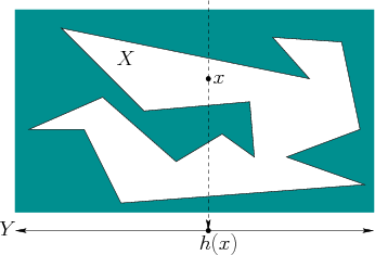
The graph example can be generalized substantially to reflect a wide variety of problems that occur in robotics and other areas. For example, Figure 11.22 shows a polygon in which a point can move. Only one coordinate is observed, and the resulting nondeterministic I-space has layers similar to those obtained for Example 11.21. These ideas can be generalized to any dimension. Interesting models can be constructed using the simple projection sensors, such as a position sensor or compass, from Section 11.5.1. In Section 12.4, such layers will appear in a pursuit-evasion game that uses visibility sensors to find moving targets.