2.3.3 Dijkstra Revisited

So far two different kinds of dynamic programming have been covered. The value-iteration method of Section 2.3.2 involves repeated computations over the entire state space. Dijkstra's algorithm from Section 2.2.2 flows only once through the state space, but with the additional overhead of maintaining which states are alive.

Dijkstra's algorithm can be derived by focusing on the forward value iterations, as in Example 2.5, and identifying exactly where the ``interesting'' changes occur. Recall that for Dijkstra's algorithm, it was assumed that all costs are nonnegative. For any states that are not reachable, their values remain at infinity. They are precisely the unvisited states. States for which the optimal cost-to-come has already become stationary are dead. For the remaining states, an initial cost is obtained, but this cost may be lowered one or more times until the optimal cost is obtained. All states for which the cost is finite, but possibly not optimal, are in the queue, ${Q}$.

After understanding value iteration, it is easier to understand why Dijkstra's form of dynamic programming correctly computes optimal solutions. It is clear that the unvisited states will remain at infinity in both algorithms because no plan has reached them. It is helpful to consider the forward value iterations in Example 2.5 for comparison. In a sense, Dijkstra's algorithm is very much like the value iteration, except that it efficiently maintains the set of states within which cost-to-go values can change. It correctly inserts any states that are reached for the first time, changing their cost-to-come from infinity to a finite value. The values are changed in the same manner as in the value iterations. At the end of both algorithms, the resulting values correspond to the stationary, optimal cost-to-come, $C^*$.

If Dijkstra's algorithm seems so clever, then why have we spent time covering the value-iteration method? For some problems it may become too expensive to maintain the sorted queue, and value iteration could provide a more efficient alternative. A more important reason is that value iteration extends easily to a much broader class of problems. Examples include optimal planning over continuous state spaces (Sections 8.5.2 and 14.5), stochastic optimal planning (Section 10.2), and computing dynamic game equilibria (Section 10.5). In some cases, it is still possible to obtain a Dijkstra-like algorithm by focusing the computation on the ``interesting'' region; however, as the model becomes more complicated, it may be inefficient or impossible in practice to maintain this region. Therefore, it is important to have a good understanding of both algorithms to determine which is most appropriate for a given problem.

Figure 2.16: A generalization of Dijkstra's algorithm, which upon termination produces an optimal plan (if one exists) for any prioritization of ${Q}$, as long as $X$ is finite. Compare this to Figure 2.4.

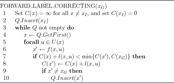
Dijkstra's algorithm belongs to a broader family of label-correcting algorithms, which all produce optimal plans by making small modifications to the general forward-search algorithm in Figure 2.4. Figure 2.16 shows the resulting algorithm. The main difference is to allow states to become alive again if a better cost-to-come is found. This enables other cost-to-come values to be improved accordingly. This is not important for Dijkstra's algorithm and $A^*$ search because they only need to visit each state once. Thus, the algorithms in Figures 2.4 and 2.16 are essentially the same in this case. However, the label-correcting algorithm produces optimal solutions for any sorting of ${Q}$, including FIFO (breadth first) and LIFO (depth first), as long as $X$ is finite. If $X$ is not finite, then the issue of systematic search dominates because one must guarantee that states are revisited sufficiently many times to guarantee that optimal solutions will eventually be found.

Another important difference between label-correcting algorithms and the standard forward-search model is that the label-correcting approach uses the cost at the goal state to prune away many candidate paths; this is shown in line 7. Thus, it is only formulated to work for a single goal state; it can be adapted to work for multiple goal states, but performance degrades. The motivation for including $C({x_{G}})$ in line 7 is that there is no need to worry about improving costs at some state, $x'$, if its new cost-to-come would be higher than $C({x_{G}})$; there is no way it could be along a path that improves the cost to go to ${x_{G}}$. Similarly, ${x_{G}}$ is not inserted in line 10 because there is no need to consider plans that have ${x_{G}}$ as an intermediate state. To recover the plan, either pointers can be stored from $x$ to $x'$ each time an update is made in line 7, or the final, optimal cost-to-come, $C^*$, can be used to recover the actions using (2.20).