Next: 9.5.2.3 Incorrect assumptions on Up: 9.5.2 Concerns Regarding the Previous: 9.5.2.1 Bayesians vs. frequentists
Suppose that the Bayesian method has been adopted. The most
widespread concern in all Bayesian analyses is the source of the prior
distribution. In Section 9.2, this is represented as
![]() (or
(or ![]() ), which represents a distribution (or
density) over the nature action space. The best way to obtain
), which represents a distribution (or
density) over the nature action space. The best way to obtain
![]() is by estimating the distribution over numerous
independent trials. This brings its definition into alignment with
frequentist views. This was possible with Example 9.11, in
which
is by estimating the distribution over numerous
independent trials. This brings its definition into alignment with
frequentist views. This was possible with Example 9.11, in
which ![]() could be reliably estimated from the frequency of
occurrence of letters across numerous pages of text. The distribution
could even be adapted to a particular language or theme.
could be reliably estimated from the frequency of
occurrence of letters across numerous pages of text. The distribution
could even be adapted to a particular language or theme.
In most applications that use decision theory, however, it is impossible or too costly to perform such experiments. What should be done in this case? If a prior distribution is simply ``made up,'' then the resulting posterior probabilities may be suspect. In fact, it may be invalid to call them probabilities at all. Sometimes the term subjective probabilities is used in this case. Nevertheless, this is commonly done because there are few other options. One of these options is to resort to frequentist decision theory, but, as mentioned, it does not work with single observations.
Fortunately, as the number of observations increases, the influence of
the prior on the Bayesian posterior distributions diminishes. If
there is only one observation, or even none as in Formulation
9.3, then the prior becomes very influential. If there
is little or no information regarding ![]() , the distribution
should be designed as carefully as possible. It should also be
understood that whatever conclusions are made with this assumption,
they are biased by the prior. Suppose this model is used as the basis
of a planning approach. You might feel satisfied computing the
``optimal'' plan, but this notion of optimality could still depend on
some arbitrary initial bias due to the assignment of prior values.
, the distribution
should be designed as carefully as possible. It should also be
understood that whatever conclusions are made with this assumption,
they are biased by the prior. Suppose this model is used as the basis
of a planning approach. You might feel satisfied computing the
``optimal'' plan, but this notion of optimality could still depend on
some arbitrary initial bias due to the assignment of prior values.
If there is no information available, then it seems reasonable that
![]() should be as uniform as possible over
should be as uniform as possible over ![]() . This was
referred to by Laplace as the ``principle of insufficient reason''
[581]. If there is no reason to believe that one element is
more likely than another, then they should be assigned equal values.
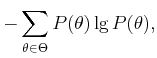
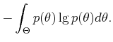
This can also be justified by using Shannon's entropy measure from
information theory [49,248,864]. In the discrete case,
this is
. This was
referred to by Laplace as the ``principle of insufficient reason''
[581]. If there is no reason to believe that one element is
more likely than another, then they should be assigned equal values.
This can also be justified by using Shannon's entropy measure from
information theory [49,248,864]. In the discrete case,
this is
It turns out that the entropy function is maximized when ![]() is a uniform distribution, which seems to justify the principle of
insufficient reason. This can be considered as a noninformative
prior. The idea is even applied quite frequently when
is a uniform distribution, which seems to justify the principle of
insufficient reason. This can be considered as a noninformative
prior. The idea is even applied quite frequently when
![]() , which leads to an improper prior. The density function
cannot maintain a constant, nonzero value over all of
, which leads to an improper prior. The density function
cannot maintain a constant, nonzero value over all of
![]() because
its integral would be infinite. Since the decisions made in Section
9.2 do not depend on any normalizing factors, a constant
value can be assigned for
because
its integral would be infinite. Since the decisions made in Section
9.2 do not depend on any normalizing factors, a constant
value can be assigned for ![]() and the decisions are not
affected by the fact that the prior is improper.
and the decisions are not
affected by the fact that the prior is improper.
The main difficulty with applying the entropy argument in the
selection of a prior is that ![]() itself may be chosen in a number
of arbitrary ways. Uniform assignments to different choices of
itself may be chosen in a number
of arbitrary ways. Uniform assignments to different choices of
![]() ultimately yield different information regarding the priors.
Consider the following example.
ultimately yield different information regarding the priors.
Consider the following example.
After thinking more carefully, perhaps we would like to distinguish
between different kinds of precipitation. A better set of nature
actions would be
![]() , in which
, in which ![]() still means
``clear,'' but precipitation
still means
``clear,'' but precipitation ![]() has been divided into
has been divided into ![]() for
``rain'' and
for
``rain'' and ![]() for ``snow.'' Now maximizing (9.89)
assigns probability
for ``snow.'' Now maximizing (9.89)
assigns probability ![]() to each nature action. This is clearly
different from the original assignment. Now that we distinguish
between different kinds of precipitation, it seems that precipitation
is much more likely to occur. Does our preference to distinguish
between different forms of precipitation really affect the weather?
to each nature action. This is clearly
different from the original assignment. Now that we distinguish
between different kinds of precipitation, it seems that precipitation
is much more likely to occur. Does our preference to distinguish
between different forms of precipitation really affect the weather?
![]()
What initial probability density should be assigned to ![]() , the
set of all lines? Suppose that the line lives in
, the
set of all lines? Suppose that the line lives in
![]() . The
line equation can be expressed as
. The
line equation can be expressed as
In some settings, there is a natural representation of the parameter
space that is invariant to certain transformations. Section
5.1.4 introduced the notion of Haar measure. If the
Haar measure is used as a noninformative prior, then a meaningful
notion of uniformity may be obtained. For example, suppose that the
parameter space is ![]() . Uniform probability mass over the space
of unit quaternions, as suggested in Example 5.14, is an
excellent choice for a noninformative prior because it is consistent
with the Haar measure, which is invariant to group operations applied
to the events. Unfortunately, a Haar measure does not exist for most
spaces that arise in practice.9.9
. Uniform probability mass over the space
of unit quaternions, as suggested in Example 5.14, is an
excellent choice for a noninformative prior because it is consistent
with the Haar measure, which is invariant to group operations applied
to the events. Unfortunately, a Haar measure does not exist for most
spaces that arise in practice.9.9
![]()
Steven M LaValle 2020-08-14