Next: Stepping along Up: 7.4.1 Adaptation of Motion Previous: Combinatorial methods
Most of the methods of Chapter 5 are not easy to
adapt because they require sampling in
![]() , for which a
parameterization does not exist. If points in a bounded region of
, for which a
parameterization does not exist. If points in a bounded region of
![]() are chosen at random, the probability is zero that a point on
are chosen at random, the probability is zero that a point on
![]() will be obtained. Some incremental sampling and searching
methods can, however, be adapted by the construction of a local
planning method (LPM) that is suited for problems with closure
constraints. The sampling-based roadmap methods require many samples
to be generated directly on
will be obtained. Some incremental sampling and searching
methods can, however, be adapted by the construction of a local
planning method (LPM) that is suited for problems with closure
constraints. The sampling-based roadmap methods require many samples
to be generated directly on
![]() . Section 7.4.2
presents some techniques that can be used to generate such samples for
certain classes of problems, enabling the development of efficient
sampling-based planners and also improving the efficiency of
incremental search planners. Before covering these techniques, we
first present a method that leads to a more general sampling-based
planner and is easier to implement. However, if designed well,
planners based on the techniques of Section 7.4.2 are more
efficient.
. Section 7.4.2
presents some techniques that can be used to generate such samples for
certain classes of problems, enabling the development of efficient
sampling-based planners and also improving the efficiency of
incremental search planners. Before covering these techniques, we
first present a method that leads to a more general sampling-based
planner and is easier to implement. However, if designed well,
planners based on the techniques of Section 7.4.2 are more
efficient.
 |
Now consider adapting the RDT of
Section 5.5 to work for problems with closure constraints.
Similar adaptations may be possible for other incremental sampling and
searching methods covered in Section 5.4, such as the
randomized potential field planner. A dense sampling sequence,
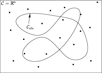
![]() , is generated over a bounded
, is generated over a bounded ![]() -dimensional subset of
-dimensional subset of
![]() , such as a rectangle or sphere, as shown in Figure
7.21. The samples are not actually required to lie on
, such as a rectangle or sphere, as shown in Figure
7.21. The samples are not actually required to lie on
![]() because they do not necessarily become part of the topological
graph,
because they do not necessarily become part of the topological
graph, ![]() . They mainly serve to pull the search tree in
different directions. One concern in choosing the bounding region is
that it must include
. They mainly serve to pull the search tree in
different directions. One concern in choosing the bounding region is
that it must include
![]() (at least the connected component that
includes
(at least the connected component that
includes ![]() ) but it must not be unnecessarily large. Such
bounds are obtained by analyzing the motion limits for a particular
linkage.
) but it must not be unnecessarily large. Such
bounds are obtained by analyzing the motion limits for a particular
linkage.
 |
Steven M LaValle 2020-08-14