Next: A zero-dimensional variety Up: 4.4.2 Kinematic Chains in Previous: 4.4.2 Kinematic Chains in
If there are two links,
![]() and
and
![]() , then the C-space can be
nicely visualized as a square with opposite faces identified. Each
coordinate,
, then the C-space can be
nicely visualized as a square with opposite faces identified. Each
coordinate, ![]() and
and ![]() , ranges from 0 to
, ranges from 0 to ![]() , for
which
, for
which
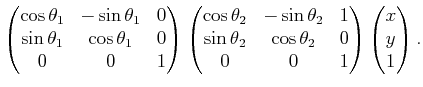
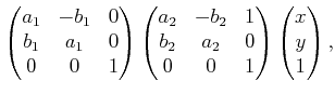
![]() . Suppose that each link has length
. Suppose that each link has length ![]() . This
yields
. This
yields ![]() . A point
. A point
![]() is transformed as
is transformed as
To obtain polynomials, the technique from Section
4.2.2 is applied to replace the trigonometric
functions using
![]() and
and
![]() , subject
to the constraint
, subject
to the constraint
![]() . This results in
. This results in
Multiplying the matrices in (4.59) yields the
polynomials,
![]() ,
,
Steven M LaValle 2020-08-14