4.3.2 Explicitly Modeling ${\cal C}_{obs}$: The Translational Case

It is important to understand how to construct a representation of ${\cal C}_{obs}$. In some algorithms, especially the combinatorial methods of Chapter 6, this represents an important first step to solving the problem. In other algorithms, especially the sampling-based planning algorithms of Chapter 5, it helps to understand why such constructions are avoided due to their complexity.

The simplest case for characterizing ${\cal C}_{obs}$ is when ${\cal C}= {\mathbb{R}}^n$ for $n = 1$, $2$, and $3$, and the robot is a rigid body that is restricted to translation only. Under these conditions, ${\cal C}_{obs}$ can be expressed as a type of convolution. For any two sets $X, Y \subset {\mathbb{R}}^n$, let their Minkowski difference^4.10 be defined as

$$X \ominus Y = \{x-y \in {\mathbb{R}}^n \;\vert\; x \in X y \in Y \},$$ (4.37)

in which $x-y$ is just vector subtraction on ${\mathbb{R}}^n$. The Minkowski difference between $X$ and $Y$ can also be considered as the Minkowski sum of $X$ and $-Y$. The Minkowski sum $\oplus$ is obtained by simply adding elements of $X$ and $Y$ in (4.37), as opposed to subtracting them. The set $-Y$ is obtained by replacing each $y \in Y$ by $-y$.

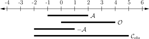
In terms of the Minkowski difference, ${\cal C}_{obs}= {\cal O}\ominus {\cal A}(0)$. To see this, it is helpful to consider a one-dimensional example.

Example 4..13 (One-Dimensional C-Space Obstacle)   In Figure 4.12, both the robot ${\cal A}= [-1,2]$ and obstacle region ${\cal O}= [0,4]$ are intervals in a one-dimensional world, ${\cal W}= {\mathbb{R}}$. The negation, $-{\cal A}$, of the robot is shown as the interval $[-2,1]$. Finally, by applying the Minkowski sum to ${\cal O}$ and $-{\cal A}$, the C-space obstacle, ${\cal C}_{obs}= [-2,5]$, is obtained. $\blacksquare$

Figure 4.12: A one-dimensional C-space obstacle.

The Minkowski difference is often considered as a convolution. It can even be defined to appear the same as studied in differential equations and system theory. For a one-dimensional example, let $f : {\mathbb{R}}\rightarrow \{0,1\}$ be a function such that $f(x) = 1$ if and only if $x \in {\cal O}$. Similarly, let $g : {\mathbb{R}}\rightarrow \{0,1\}$ be a function such that $g(x) = 1$ if and only if $x \in {\cal A}$. The convolution

$$h(x) = \int_{-\infty}^{\infty} f(\tau) g(x - \tau) d\tau ,$$ (4.38)

yields a function $h$, for which $h(x)>0$ if $x \in \operatorname{int}({\cal C}_{obs})$, and $h(x) = 0$ otherwise.